Model Construction and Training
This chapter describes how to build models with Keras and Eager Execution using TensorFlow 2.
Model construction:
tf.keras.Modelandtf.keras.layersLoss function of the model:
tf.keras.lossesOptimizer of the model:
tf.keras.optimizerEvaluation of models:
tf.keras.metrics
Prerequisite
Object-oriented Python programming (define classes and methods, class inheritance, constructor and deconstructor within Python, use super() functions to call parent class methods, use __call__() methods to call instances, etc.).
Multilayer perceptron, convolutional neural networks, recurrent neural networks and reinforcement learning (references given before each section).
Python function decorator (not required)
Models and layers
In TensorFlow, it is recommended to build models using Keras (tf.keras), a popular high-level neural network API that is simple, fast and flexible. It is officially built-in and fully supported by TensorFlow.
There are two important concepts in Keras: Model and Layer . The layers encapsulate various computational processes and variables (e.g., fully connected layers, convolutional layers, pooling layers, etc.), while the model connects the layers and encapsulates them as a whole, describing how the input data is passed through the layers and operations to get the output. Keras has built in a number of predefined layers commonly used in deep learning under tf.keras.layers, while also allowing us to customize the layers.
Keras models are presented as classes, and we can define our own models by inheriting the Python class tf.keras.Model. In the inheritance class, we need to rewrite the __init__() (constructor) and call(input) (model call) methods, but we can also add custom methods as needed.
class MyModel(tf.keras.Model):
    def __init__(self):
        super().__init__()
        # Add initialization code here, including the layers that will be used in call(). e.g.,
        # layer1 = tf.keras.layers.BuiltInLayer(...)
        # layer2 = MyCustomLayer(...)

    def call(self, input):
        # Add the code for the model call here (process the input and return the output). e.g.,
        # x = layer1(input)
        # output = layer2(x)
        return output

    # add your custom methods here
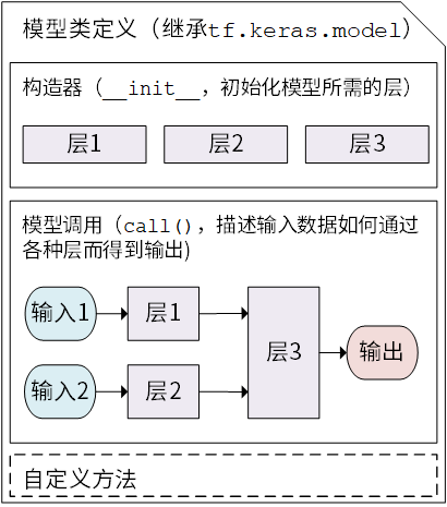
Keras model class structure
After inheriting tf.keras.Model, we can use several methods and properties of the parent class at the same time. For example, after instantiating the class model = Model(), we can get all the variables in the model directly through the property model.variables, saving us from the trouble of specifying them one by one explicitly.
Then, we can rewrite the simple linear model in the previous chapter y_pred = a * X + b with Keras model class as follows
import tensorflow as tf

X = tf.constant([[1.0, 2.0, 3.0], [4.0, 5.0, 6.0]])
y = tf.constant([[10.0], [20.0]])


class Linear(tf.keras.Model):
    def __init__(self):
        super().__init__()
        self.dense = tf.keras.layers.Dense(
            units=1,
            activation=None,
            kernel_initializer=tf.zeros_initializer(),
            bias_initializer=tf.zeros_initializer()
        )

    def call(self, input):
        output = self.dense(input)
        return output


# 以下代码结构与前节类似
model = Linear()
optimizer = tf.keras.optimizers.SGD(learning_rate=0.01)
for i in range(100):
    with tf.GradientTape() as tape:
        y_pred = model(X)      # 调用模型 y_pred = model(X) 而不是显式写出 y_pred = a * X + b
        loss = tf.reduce_mean(tf.square(y_pred - y))
    grads = tape.gradient(loss, model.variables)    # 使用 model.variables 这一属性直接获得模型中的所有变量
    optimizer.apply_gradients(grads_and_vars=zip(grads, model.variables))
print(model.variables)
Here, instead of explicitly declaring two variables a and b and writing the linear transformation y_pred = a * X + b, we create a model class Linear that inherits tf.keras.Model. This class instantiates a fully connected layer (tf.keras.layers.Dense`) in the constructor, and calls this layer in the call method, implementing the calculation of the linear transformation. If you need to explicitly declare your own variables and use them for custom operations, or want to understand the inner workings of the Keras layer, see Custom Layer.
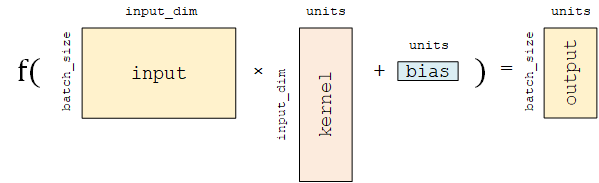
Fully connection layer in Keras: linear transformation + activation function
Fully-connected Layer (tf.keras.layers.Dense) is one of the most basic and commonly used layers in Keras, which performs a linear transformation and activation  on the input matrix
  . If the activation function is not specified, it is a purely linear transformation
  . Specifically, for a given input tensor
 input = [match_size, input_dim] , the layer first performs a linear transformation on the input tensor tf.matmul(input, kernel) + bias (kernel and bias are trainable variables in the layer), and then apply the activation function activation on each element of the linearly transformed tensor, thereby outputting a two-dimensional tensor with shape [match_size, units].
tf.keras.layers.Dense contains the following main parameters.
units: the dimension of the output tensor.activation: the activation function, corresponding to in (Default: no activation). Commonly used activation functions include
 tf.nn.relu,tf.nn.tanhandtf.nn.sigmoid.use_bias: whether to add the bias vectorbias, i.e. in (Default:
 True).kernel_initializer,bias_initializer: initializer of the two variables, the weight matrixkerneland the bias vectorbias. The default istf.glorot_uniform_initializer1. Set them totf.zeros_initializermeans that both variables are initialized to zero tensors.
This layer contains two trainable variables, the weight matrix kernel = [input_dim, units] and the bias vector bias = [bits] 2 , corresponding to  and in .
The fully connected layer is described here with emphasis on mathematical matrix operations. A description of neuron-based modeling can be found here.
- 1
Many layers in Keras use
tf.glorot_uniform_initializerby default to initialize variables, which can be found at https://www.tensorflow.org/api_docs/python/tf/glorot_uniform_initializer.- 2
You may notice that
tf.matmul(input, kernel)results in a two-dimensional matrix with shape[batch_size, units]. How is this two-dimensional matrix to be added to the one-dimensional bias vectorbiaswith shape[units]? In fact, here is TensorFlow’s Broadcasting mechanism at work. The add operation is equivalent to addingbiasto each row of the two-dimensional matrix. A detailed description of the Broadcasting mechanism can be found at https://www.tensorflow.org/xla/broadcasting.
Why is the model class override call() instead of __call__()?
In Python, a call to an instance of a class myClass (i.e., myClass(params)) is equivalent to myClass.__call__(params) (see the __call__() part of “Prerequisite” at the beginning of this chapter). Then in order to call the model using y_pred = model(X), it seems that one should override the __call__() method instead of call(). Why we do the opposite? The reason is that Keras still needs to have some pre-processing and post-processing for the model call, so it is more reasonable to expose a call() method specifically for overriding. The parent class tf.keras.Model already contains the definition of __call__(). The call() method is invoked in __call__() while some internal operations of the keras are also performed. Therefore, by inheriting the tf.keras.Model and overriding the call() method, we can add the code of model call while maintaining the inner structure of Keras.
Basic example: multi-layer perceptron (MLP)
We use the simplest multilayer perceptron (MLP), or “multilayer fully connected neural network” as an example to introduce the model building process in TensorFlow 2. In this section, we take the following steps
Acquisition and pre-processing of datasets using
tf.keras.datasetsModel construction using
tf.keras.Modelandtf.keras.layersBuild model training process. Use
tf.keras.losesto calculate loss functions and usetf.keras.optimizerto optimize modelsBuild model evaluation process. Use
tf.keras.metricsto calculate assessment indicators (e.g., accuracy)
Basic knowledges and principles
The Multi-Layer Neural Network section of the UFLDL tutorial.
“Neural Networks Part 1 ~ 3” section of the Stanford course CS231n: Convolutional Neural Networks for Visual Recognition.
Here, we use a multilayer perceptron to tackle the classification task on the MNIST handwritten digit dataset [LeCun1998].
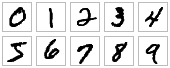
examples of MNIST handwritten digit
Data acquisition and pre-processing with tf.keras.datasets
To prepare the data, we first implement a simple MNISTLoader class to read data from the MNIST dataset. tf.keras.datasets are used here to simplify the download and loading process of MNIST dataset.
class MNISTLoader():
    def __init__(self):
        mnist = tf.keras.datasets.mnist
        (self.train_data, self.train_label), (self.test_data, self.test_label) = mnist.load_data()
        # MNIST中的图像默认为uint8(0-255的数字)。以下代码将其归一化到0-1之间的浮点数,并在最后增加一维作为颜色通道
        self.train_data = np.expand_dims(self.train_data.astype(np.float32) / 255.0, axis=-1)      # [60000, 28, 28, 1]
        self.test_data = np.expand_dims(self.test_data.astype(np.float32) / 255.0, axis=-1)        # [10000, 28, 28, 1]
        self.train_label = self.train_label.astype(np.int32)    # [60000]
        self.test_label = self.test_label.astype(np.int32)      # [10000]
        self.num_train_data, self.num_test_data = self.train_data.shape[0], self.test_data.shape[0]

    def get_batch(self, batch_size):
        # 从数据集中随机取出batch_size个元素并返回
        index = np.random.randint(0, self.num_train_data, batch_size)
        return self.train_data[index, :], self.train_label[index]
Hint
mnist = tf.keras.datasets.mnist will automatically download and load the MNIST data set from the Internet. If a network connection error occurs at runtime, you can download the MNIST dataset mnist.npz manually from https://storage.googleapis.com/tensorflow/tf-keras-datasets/mnist.npz or https://s3.amazonaws.com/img-datasets/mnist.npz ,and move it into the .keras/dataset directory of the user directory (C:\Users\USERNAME for Windows and /home/USERNAME for Linux).
Image data representation in TensorFlow
In TensorFlow, a typical representation of an image data set is a four-dimensional tensor of [number of images, width, height, number of color channels]. In the DataLoader class above, self.train_data and self.test_data were loaded with 60,000 and 10,000 handwritten digit images of size 28*28, respectively. Since we are reading a grayscale image here with only one color channel (a regular RGB color image has 3 color channels), we use the np.expand_dims() function to manually add one dimensional channels at the last dimension for the image data.
Model construction with tf.keras.Model and tf.keras.layers
The implementation of the multi-layer perceptron is similar to the linear model above, constructed using tf.keras.Model and tf.keras.layers, except that the number of layers is increased (as the name implies, “multi-layer” perceptron), and a non-linear activation function is introduced (here we use the ReLU function activation function, i.e. activation=tf.nn.relu below). The model accepts a vector (e.g. here a flattened 1×784 handwritten digit image) as input and outputs a 10-dimensional vector representing the probability that this image belongs to 0 to 9 respectively.
class MLP(tf.keras.Model):
    def __init__(self):
        super().__init__()
        self.flatten = tf.keras.layers.Flatten()    # Flatten层将除第一维(batch_size)以外的维度展平
        self.dense1 = tf.keras.layers.Dense(units=100, activation=tf.nn.relu)
        self.dense2 = tf.keras.layers.Dense(units=10)

    def call(self, inputs):         # [batch_size, 28, 28, 1]
        x = self.flatten(inputs)    # [batch_size, 784]
        x = self.dense1(x)          # [batch_size, 100]
        x = self.dense2(x)          # [batch_size, 10]
        output = tf.nn.softmax(x)
        return output
Softmax function
Here, because we want to output the probabilities that the input images belongs to 0 to 9 respectively, i.e. a 10-dimensional discrete probability distribution, we want this 10-dimensional vector to satisfy at least two conditions.
Each element in the vector is between
![[0, 1]](../../_images/math/1a9360a164e54bf10a49ee770650287ce1e13124.png) .
.The sum of all elements of the vector is 1.
To ensure the output of the model to always satisfy both conditions, we normalize the raw output of the model using the Softmax function (normalized exponential function, tf.nn.softmax). Its mathematical form is 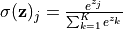 . Not only that, the softmax function is able to highlight the largest value in the original vector and suppress other components that are far below the maximum, which is why it is called the softmax function (that is, the smoothed argmax function).
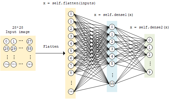
MLP model
Model training with tf.keras.losses and tf.keras.optimizer
To train the model, first we define some hyperparameters of the model used in training process
num_epochs = 5
batch_size = 50
learning_rate = 0.001
Then, we instantiate the model and data reading classes, and instantiate an optimizer in tf.keras.optimizer (the Adam optimizer is used here).
model = MLP()
data_loader = MNISTLoader()
optimizer = tf.keras.optimizers.Adam(learning_rate=learning_rate)
The following steps are then iterated.
A random batch of training data is taken from the DataLoader.
Feed the data into the model, and obtain the predicted value from the model.
Calculate the loss function (
loss) by comparing the model predicted value with the true value. Here we use the cross-entropy function intf.keras.lossesas a loss function.Calculate the derivative of the loss function on the model variables (gradients).
The derivative values (gradients) are passed into the optimizer, and use the
apply_gradientsmethod to update the model variables so that the loss value is minimized (see previous chapter for details on how to use the optimizer).
The code is as follows
    num_batches = int(data_loader.num_train_data // batch_size * num_epochs)
    for batch_index in range(num_batches):
        X, y = data_loader.get_batch(batch_size)
        with tf.GradientTape() as tape:
            y_pred = model(X)
            loss = tf.keras.losses.sparse_categorical_crossentropy(y_true=y, y_pred=y_pred)
            loss = tf.reduce_mean(loss)
            print("batch %d: loss %f" % (batch_index, loss.numpy()))
        grads = tape.gradient(loss, model.variables)
        optimizer.apply_gradients(grads_and_vars=zip(grads, model.variables))
Cross entropy and tf.keras.losses
You may notice that, instead of explicitly writing a loss function, we use the sparse_categorical_crossentropy (cross entropy) function in tf.keras.losses. We pass the model predicted value y_pred and the real value y_true into the function as parameters, then this Keras function helps us calculate the loss value.
Cross-entropy is widely used as a loss function in classification problems. The discrete form is  , where
  is the true probability distribution,
  is the predicted probability distribution, and
  is the number of categories in the classification task. The closer the predicted probability distribution is to the true distribution, the smaller the value of the cross-entropy, and vice versa. A more specific introduction and its application to machine learning can be found in this blog post.
In tf.keras, there are two cross-entropy related loss functions tf.keras.losses.categorical_crossentropy and tf.keras.losses.sparse_categorical_crossentropy. Here “sparse” means that the true label value y_true can be passed directly into the function as integer. That means,
loss = tf.keras.losses.sparse_categorical_crossentropy(y_true=y, y_pred=y_pred)
is equivalent to
loss = tf.keras.losses.categorical_crossentropy(
    y_true=tf.one_hot(y, depth=tf.shape(y_pred)[-1]),
    y_pred=y_pred
)
Model Evaluation with tf.keras.metrics
Finally, we use the test set to evaluate the performance of the model. Here, we use the SparseCategoricalAccuracy metric in tf.keras.metrics to evaluate the performance of the model on the test set, which compares the results predicted by the model with the true results, and outputs the proportion of the test data samples that is correctly classified by the model. We do evaluatio iteratively on the test set, feeding the results predicted by the model and the true results into the metric instance each time by the update_state() method, with two parameters y_pred and y_true respectively. The metric instance has internal variables to maintain the values associated with the current evaluation process (e.g., the current cumulative number of samples that has been passed in and the current number of samples that predicts correctly). At the end of the iteration, we use the result() method to output the final evaluation value (the proportion of the correctly classified samples over the total samples).
In the following code, we instantiate a tf.keras.metrics.SparseCategoricalAccuracy metric, use a for loop to feed the predicted and true results iteratively, and output the accuracy of the trained model on the test set.
    sparse_categorical_accuracy = tf.keras.metrics.SparseCategoricalAccuracy()
    num_batches = int(data_loader.num_test_data // batch_size)
    for batch_index in range(num_batches):
        start_index, end_index = batch_index * batch_size, (batch_index + 1) * batch_size
        y_pred = model.predict(data_loader.test_data[start_index: end_index])
        sparse_categorical_accuracy.update_state(y_true=data_loader.test_label[start_index: end_index], y_pred=y_pred)
    print("test accuracy: %f" % sparse_categorical_accuracy.result())
Output:
test accuracy: 0.947900
It can be noted that we can reach an accuracy rate of around 95% just using such a simple model.
The basic unit of a neural network: the neuron 3
If we take a closer look at the neural network above and study the computational process in detail, for example by taking the k-th computational unit of the second layer, we can get the following schematic
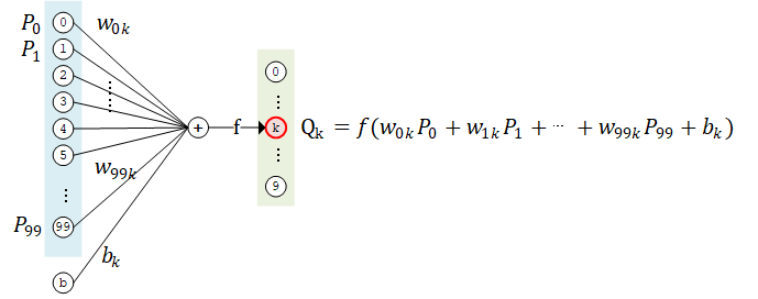
The computational unit  has 100 weight parameters
  and 1 bias parameter
  . The values of
  of all 100 computational units in layer 1 are taken as inputs, summed by weight
  (i.e.
(i.e.  ) and biased by , then it is fed into the activation function to get the output result.
In fact, this structure is quite similar to real nerve cells (neurons). Neurons are composed of dendrites, cytosomes and axons. Dendrites receive signals from other neurons as input (one neuron can have thousands or even tens of thousands of dendrites), the cell body integrates the potential signal, and the resulting signal travels through axons to synapses at nerve endings and propagates to the next (or more) neuron.
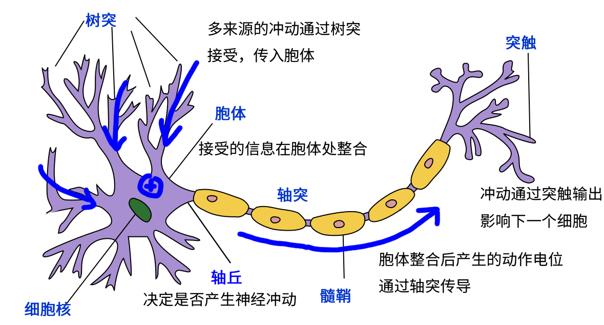
Neural cell pattern diagram (modified from Quasar Jarosz at English Wikipedia [CC BY-SA 3.0 (https://creativecommons.org/licenses/by-sa/3.0)])
The computational unit above can be viewed as a mathematical modeling of neuronal structure. In the above example, each computational unit (artificial neuron) in the second layer has 100 weight parameters and 1 bias parameter, while the number of computational units in the second layer is 10, so the total number of participants in this fully connected layer is 100*10 weight parameters and 10 bias parameters. In fact, this is the shape of the two variables kernel and bias in this fully connected layer. Upon closer examination, you will see that the introduction to neuron-based modeling here is equivalent to the introduction to matrix-based computing above.
- 3
Actually, there should be the concept of neuronal modeling first, followed by artificial neural networks based on artificial neurons and layer structures. However, since this manual focuses on how to use TensorFlow, the order of introduction is switched.
Convolutional Neural Network (CNN)
Convolutional Neural Network (CNN) is an artificial neural network with a structure similar to the visual system of a human or animal, that contains one or more Convolutional Layer, Pooling Layer and Fully-connected Layer.
Basic knowledges and principles
Convolutional Neural Network in UFLDL Tutorial
“Module 2: Convolutional Neural Networks” in Stanford course CS231n: Convolutional Neural Networks for Visual Recognition
“Convolutional Neural Networks” in Dive into Deep Learning
Implementing Convolutional Neural Networks with Keras
An example implementation of a convolutional neural network is shown below. The code structure is similar to the multi-layer perceptron in the previous section, except that some new convolutional and pooling layers are added. The network structure here is not unique: the layers in the CNN can be added, removed or adjusted for better performance.
class CNN(tf.keras.Model):
    def __init__(self):
        super().__init__()
        self.conv1 = tf.keras.layers.Conv2D(
            filters=32,             # 卷积层神经元(卷积核)数目
            kernel_size=[5, 5],     # 感受野大小
            padding='same',         # padding策略(vaild 或 same)
            activation=tf.nn.relu   # 激活函数
        )
        self.pool1 = tf.keras.layers.MaxPool2D(pool_size=[2, 2], strides=2)
        self.conv2 = tf.keras.layers.Conv2D(
            filters=64,
            kernel_size=[5, 5],
            padding='same',
            activation=tf.nn.relu
        )
        self.pool2 = tf.keras.layers.MaxPool2D(pool_size=[2, 2], strides=2)
        self.flatten = tf.keras.layers.Reshape(target_shape=(7 * 7 * 64,))
        self.dense1 = tf.keras.layers.Dense(units=1024, activation=tf.nn.relu)
        self.dense2 = tf.keras.layers.Dense(units=10)

    def call(self, inputs):
        x = self.conv1(inputs)                  # [batch_size, 28, 28, 32]
        x = self.pool1(x)                       # [batch_size, 14, 14, 32]
        x = self.conv2(x)                       # [batch_size, 14, 14, 64]
        x = self.pool2(x)                       # [batch_size, 7, 7, 64]
        x = self.flatten(x)                     # [batch_size, 7 * 7 * 64]
        x = self.dense1(x)                      # [batch_size, 1024]
        x = self.dense2(x)                      # [batch_size, 10]
        output = tf.nn.softmax(x)
        return output
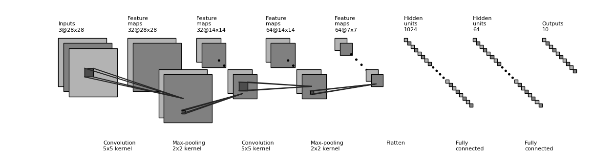
CNN structure diagram in the above sample code
Replace the code line model = MLP() in previous MLP section to model = CNN() , the output will be as follows:
test accuracy: 0.988100
A very significant improvement of accuracy can be found compared to MLP in the previous section. In fact, there is still room for further improvements by changing the network structure of the model (e.g. by adding a Dropout layer to prevent overfitting).
Using predefined classical CNN structures in Keras
There are some pre-defined classical convolutional neural network structures in tf.keras.applications, such as VGG16, VGG19, ResNet and MobileNet. We can directly apply these classical convolutional neural network (and load pre-trained weights) without manually defining the CNN structure.
For example, we can use the following code to instantiate a MobileNetV2 network structure.
model = tf.keras.applications.MobileNetV2()
When the above code is executed, TensorFlow will automatically download the pre-trained weights of the MobileNetV2 network, so Internet connection is required for the first execution of the code. You can also initialize variables randomly by setting the parameter weights to None. Each network structure has its own specific detailed parameter settings. Some shared common parameters are as follows.
input_shape: the shape of the input tensor (without the first batch dimension), which mostly defaults to224 × 224 × 3. In general, models have lower bounds on the size of the input tensor, with a minimum length and width of32 × 32or75 × 75.include_top: whether the fully-connected layer is included at the end of the network, which defaults toTrue.weights: pre-trained weights, which default toimagenet(using pre-trained weights trained on ImageNet dataset). It can be set toNoneif you want to randomly initialize the variables.classes: the number of classes, which defaults to 1000. If you want to modify this parameter, theinclude_topparameter has to beTrueand theweightsparameter has to beNone.
A detailed description of each network model parameter can be found in the Keras documentation.
Set learning phase
For some pre-defined classical models, some of the layers (e.g. BatchNormalization) behave differently on training and testing stage (see this article). Therefore, when training this kind of model, you need to set the learning phase manually, telling the model “I am in the training stage of the model”. This can be done through
tf.keras.backend.set_learning_phase(True)
or by setting the training parameter to True when the model is called.
An example is shown below, using MobileNetV2 network to train on tf_flowers five-classifying datasets (for the sake of code brevity and efficiency, we use TensorFlow Datasets and tf.data to load and preprocess the data in this example). Also we set classes to 5, corresponding to the tf_flowers dataset with 5 kind of labels.
import tensorflow as tf
import tensorflow_datasets as tfds

num_epoch = 5
batch_size = 50
learning_rate = 0.001

dataset = tfds.load("tf_flowers", split=tfds.Split.TRAIN, as_supervised=True)
dataset = dataset.map(lambda img, label: (tf.image.resize(img, (224, 224)) / 255.0, label)).shuffle(1024).batch(batch_size)
model = tf.keras.applications.MobileNetV2(weights=None, classes=5)
optimizer = tf.keras.optimizers.Adam(learning_rate=learning_rate)
for e in range(num_epoch):
    for images, labels in dataset:
        with tf.GradientTape() as tape:
            labels_pred = model(images, training=True)
            loss = tf.keras.losses.sparse_categorical_crossentropy(y_true=labels, y_pred=labels_pred)
            loss = tf.reduce_mean(loss)
            print("loss %f" % loss.numpy())
        grads = tape.gradient(loss, model.trainable_variables)
        optimizer.apply_gradients(grads_and_vars=zip(grads, model.trainable_variables))
    print(labels_pred)
In later sections (e.g. Distributed Training), we will also directly use these classicial network structures for training.
How the Convolutional and Pooling Layers Work
The Convolutional Layer, represented by tf.keras.layers.Conv2D in Keras, is a core component of CNN and has a structure similar to the visual cortex of the brain.
Recall our previously established computational model of neurons and the fully-connected layer, in which we let each neuron connect to all other neurons in the previous layer. However, this is not the case in the visual cortex. You may have learned in biology class about the concept of Receptive Field, where neurons in the visual cortex are not connected to all the neurons in the previous layer, but only sense visual signals in an area and respond only to visual stimuli in the local area.
For example, the following figure is a 7×7 single-channel image signal input.
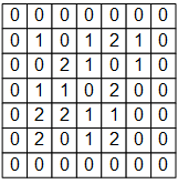
If we use the MLP model based on fully-connected layers, we need to make each input signal correspond to a weight value. In this case, modeling a neuron requires 7×7=49 weights (50 if we consider the bias) to get an output signal. If there are N neurons in a layer, we need 49N weights and get N output signals.
In the convolutional layer of CNN, we model a neuron in a convolutional layer like this.
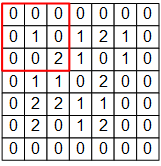
The 3×3 red box in the figure represents the receptor field of this neuron. In this case, we only need a 3×3 weight matrix 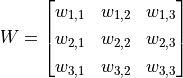 with an additional bias to get an output signal. E.g., for the red box shown in the figure, the output is the sum of all elements of matrix
 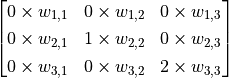 adding bias , noted as
  .
.
However, the 3×3 range is clearly not enough to handle the entire image, so we use the sliding window approach. Use the same parameter but swipe the red box from left to right in the image, scanning it line by line, calculating a value for each position it slides to. For example, when the red box moves one unit to the right, we calculate the sum of all elements of the matrix 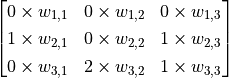 , adding bias , noted as
  . Thus, unlike normal neurons that can only output one value, the convolutional neurons here can output a 5×5 matrix
 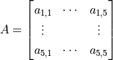 .
.
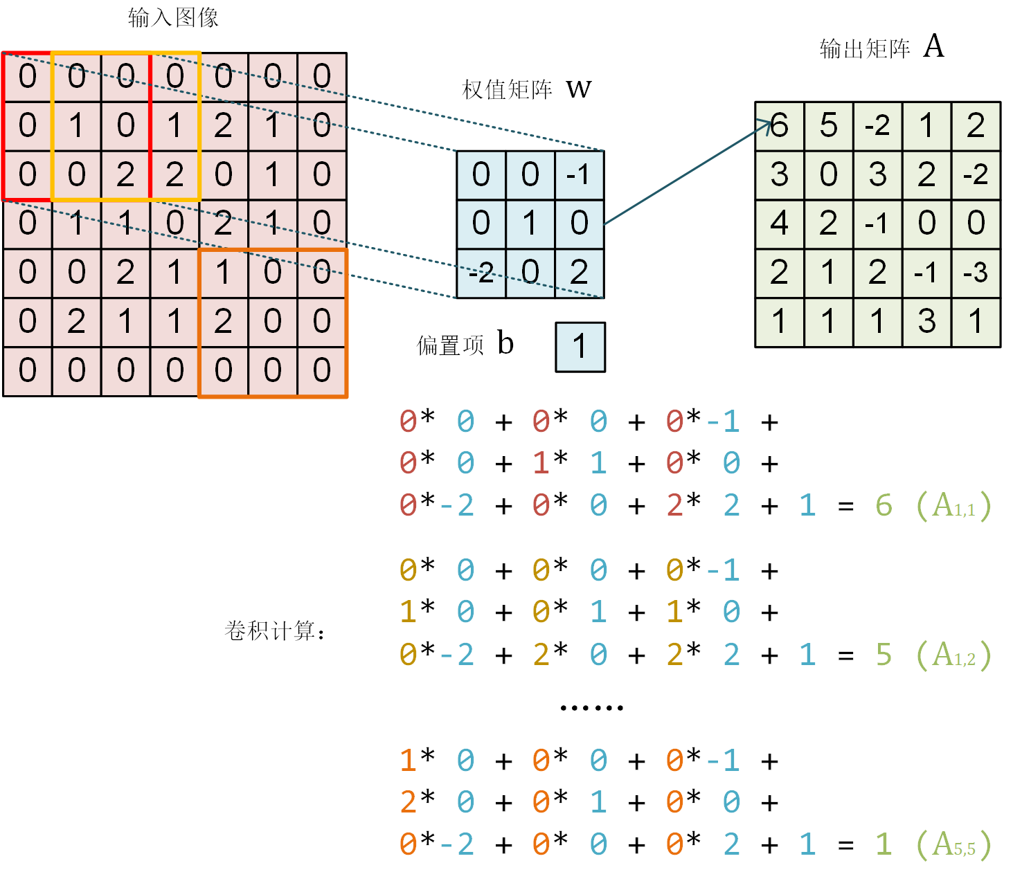
Diagram of convolution process. A single channel 7×7 image passes through a convolutional layer with a receptor field of 3×3, yielded a 5×5 matrix as result.
In the following part, we use TensorFlow to verify the results of the above calculation.
The input image, the weight matrix and the bias term in the above figure are represented as the NumPy array image, W, b as follows.
# TensorFlow 的图像表示为 [图像数目,长,宽,色彩通道数] 的四维张量
# 这里我们的输入图像 image 的张量形状为 [1, 7, 7, 1]
image = np.array([[
    [0, 0, 0, 0, 0, 0, 0],
    [0, 1, 0, 1, 2, 1, 0],
    [0, 0, 2, 2, 0, 1, 0],
    [0, 1, 1, 0, 2, 1, 0],
    [0, 0, 2, 1, 1, 0, 0],
    [0, 2, 1, 1, 2, 0, 0],
    [0, 0, 0, 0, 0, 0, 0]
]], dtype=np.float32)
image = np.expand_dims(image, axis=-1)
W = np.array([[
    [ 0, 0, -1],
    [ 0, 1, 0 ],
    [-2, 0, 2 ]
]], dtype=np.float32)
b = np.array([1], dtype=np.float32)
Then, we build a model with only one convolutional layer, initialized by W and b 4 :
model = tf.keras.models.Sequential([
    tf.keras.layers.Conv2D(
        filters=1,              # 卷积层神经元(卷积核)数目
        kernel_size=[3, 3],     # 感受野大小
        kernel_initializer=tf.constant_initializer(W),
        bias_initializer=tf.constant_initializer(b)
    )]
)
Finally, feed the image data image into the model and print the output.
output = model(image)
print(tf.squeeze(output))
The result will be
tf.Tensor(
[[ 6.  5. -2.  1.  2.]
 [ 3.  0.  3.  2. -2.]
 [ 4.  2. -1.  0.  0.]
 [ 2.  1.  2. -1. -3.]
 [ 1.  1.  1.  3.  1.]], shape=(5, 5), dtype=float32)
You can find out that this result is consistent with the value of the matrix in the figure above.
One more question, the above convolution process assumes that the images only have one channel (e.g. grayscale images), but what if the image is in color (e.g. has three channels of RGB)? Actually, we can prepare a 3×3 weight matrix for each channel, i.e. there are 3×3×3=27 weights in total. Each channel is processed using its own weight matrix, and the output can be summed by adding the values from multiple channels.
Some readers may notice that, following the method described above, the result after each convolution will be “one pixel shrinked” around. The 7×7 image above, for example, becomes 5×5 after convolution, which sometimes causes problems to the forthcoming layers. Therefore, we can set the padding strategy. In tf.keras.layers.Conv2D, when we set the padding parameter to same, the missing pixels around it are filled with 0, so that the size of the output matches the input.
Finally, since we can use the sliding window method to do convolution, can we set a different step size for the slide? The answer is yes. The step size (default is 1) can be set using the strides parameter of tf.keras.layers.Conv2D. For example, in the above example, if we set the step length to 2, the output will be a 3×3 matrix.
In fact, there are many forms of convolution, and the above introduction is only one of the simplest one. Further examples of the convolutional approach can be found in Convolution Arithmetic.
The Pooling Layer is much simpler to understand as the process of downsampling an image, outputting the maximum value (MaxPooling), the mean value, or the value generated by other methods for all values in the window for each slide. For example, for a three-channel 16×16 image (i.e., a tensor of 16*16*3), a tensor of 8*8*3 is obtained after a pooled layer with a receptive field of 2×2 and a slide step of 2.
- 4
Here we use the sequential mode to build the model for simplicity, as described later .
Recurrent Neural Network (RNN)
Recurrent Neural Network (RNN) is a type of neural network suitable for processing sequence data (especially text). It is widely used in language models, text generation and machine translation.
Basic knowledges and principles
Recurrent Neural Networks Tutorial, Part 1 – Introduction to RNNs
“Recurrent Neural Networks” in Dive into Deep Learning。
RNN sequence generation: [Graves2013]
Here, we use RNN to generate Nietzschean-style text automatically. 5
The essence of this task is to predict the probability distribution of an English sentence’s successive character. For example, we have the following sentence:
I am a studen
This sentence (sequence) has a total of 13 characters including spaces. When we read this sequence of 13 characters, we can predict based on our experience, that the next character is “t” with a high probability. Now we want to build a model to do the same thing as our experience, in which we input a sequence of seq_length one by one, and output the probability distribution of the next character that follows this sentence. Then we can generate text by sampling a character from the probability distribution as a predictive value, then do snowballing to generate the next two characters, the next three characters, etc.
First of all, we implement a simple DataLoader class to read training corpus (Nietzsche’s work) and encode it in characters. Each character is assigned a unique integer number i between 0 and num_chars - 1, in which num_chars is the number of character types.
class DataLoader():
    def __init__(self):
        path = tf.keras.utils.get_file('nietzsche.txt',
            origin='https://s3.amazonaws.com/text-datasets/nietzsche.txt')
        with open(path, encoding='utf-8') as f:
            self.raw_text = f.read().lower()
        self.chars = sorted(list(set(self.raw_text)))
        self.char_indices = dict((c, i) for i, c in enumerate(self.chars))
        self.indices_char = dict((i, c) for i, c in enumerate(self.chars))
        self.text = [self.char_indices[c] for c in self.raw_text]

    def get_batch(self, seq_length, batch_size):
        seq = []
        next_char = []
        for i in range(batch_size):
            index = np.random.randint(0, len(self.text) - seq_length)
            seq.append(self.text[index:index+seq_length])
            next_char.append(self.text[index+seq_length])
        return np.array(seq), np.array(next_char)       # [batch_size, seq_length], [num_batch]
The model implementation is carried out next. In the constructor (__init__ method), we instantiate a LSTMCell unit and a fully connected layer. in call method, We first perform a “One Hot” operation on the sequence, i.e., we transform the encoding i of each character in the sequence into a num_char dimensional vector with bit i being 1 and the rest being 0. The transformed sequence tensor has a shape of [seq_length, num_chars] . We then initialize the state of the RNN unit. Next, the characters of the sequence is fed into the RNN unit one by one. At moment t, the state of RNN unit state in the previous time step t-1 and the t-th element of the sequence inputs[t, :] are fed into the RNN unit, to get the output output and the RNN unit state in the current time step t. The last output of the RNN unit is taken and transformed through the fully connected layer to num_chars dimension.
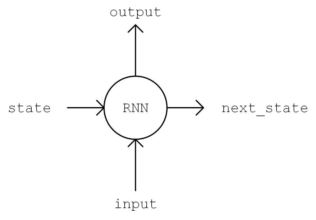
Diagram of output, state = self.cell(inputs[:, t, :], state)
RNN working process
The code implementation is like this
class RNN(tf.keras.Model):
    def __init__(self, num_chars, batch_size, seq_length):
        super().__init__()
        self.num_chars = num_chars
        self.seq_length = seq_length
        self.batch_size = batch_size
        self.cell = tf.keras.layers.LSTMCell(units=256)
        self.dense = tf.keras.layers.Dense(units=self.num_chars)

    def call(self, inputs, from_logits=False):
        inputs = tf.one_hot(inputs, depth=self.num_chars)       # [batch_size, seq_length, num_chars]
        state = self.cell.get_initial_state(batch_size=self.batch_size, dtype=tf.float32)   # 获得 RNN 的初始状态
        for t in range(self.seq_length):
            output, state = self.cell(inputs[:, t, :], state)   # 通过当前输入和前一时刻的状态,得到输出和当前时刻的状态
        logits = self.dense(output)
        if from_logits:                     # from_logits 参数控制输出是否通过 softmax 函数进行归一化
            return logits
        else:
            return tf.nn.softmax(logits)
Defining some hyperparameters of the model
    num_batches = 1000
    seq_length = 40
    batch_size = 50
    learning_rate = 1e-3
The training process is very similar to the previous section. Here we just repeat it:
A random batch of training data is taken from the DataLoader.
Feed the data into the model, and obtain the predicted value from the model.
Calculate the loss function (
loss) by comparing the model predicted value with the true value. Here we use the cross-entropy function intf.keras.lossesas a loss function.Calculate the derivative of the loss function on the model variables (gradients).
The derivative values (gradients) are passed into the optimizer, and use the
apply_gradientsmethod to update the model variables so that the loss value is minimized.
    data_loader = DataLoader()
    model = RNN(num_chars=len(data_loader.chars), batch_size=batch_size, seq_length=seq_length)
    optimizer = tf.keras.optimizers.Adam(learning_rate=learning_rate)
    for batch_index in range(num_batches):
        X, y = data_loader.get_batch(seq_length, batch_size)
        with tf.GradientTape() as tape:
            y_pred = model(X)
            loss = tf.keras.losses.sparse_categorical_crossentropy(y_true=y, y_pred=y_pred)
            loss = tf.reduce_mean(loss)
            print("batch %d: loss %f" % (batch_index, loss.numpy()))
        grads = tape.gradient(loss, model.variables)
        optimizer.apply_gradients(grads_and_vars=zip(grads, model.variables))
One thing about the process of text generation requires special attention. Previously, we have been using the tf.argmax() function, which takes the value corresponding to the maximum probability as the predicted value. For text generation, however, such predictions are too “absolute” and can make the generated text lose its richness. Thus, we use the np.random.choice() function to sample the resulting probability distribution. In this way, even characters that correspond to a small probability have a chance of being sampled. At the same time, we add a temperature parameter to control the shape of the distribution, the larger the parameter value, the smoother the distribution (the smaller the difference between the maximum and minimum values), the higher the richness of the generated text; the smaller the parameter value, the steeper the distribution, the lower the richness of the generated text.
    def predict(self, inputs, temperature=1.):
        batch_size, _ = tf.shape(inputs)
        logits = self(inputs, from_logits=True)                         # 调用训练好的RNN模型,预测下一个字符的概率分布
        prob = tf.nn.softmax(logits / temperature).numpy()              # 使用带 temperature 参数的 softmax 函数获得归一化的概率分布值
        return np.array([np.random.choice(self.num_chars, p=prob[i, :]) # 使用 np.random.choice 函数,
                         for i in range(batch_size.numpy())])           # 在预测的概率分布 prob 上进行随机取样
Through a contineous prediction of characters, we can get the automatically generated text.
    X_, _ = data_loader.get_batch(seq_length, 1)
    for diversity in [0.2, 0.5, 1.0, 1.2]:      # 丰富度(即temperature)分别设置为从小到大的 4 个值
        X = X_
        print("diversity %f:" % diversity)
        for t in range(400):
            y_pred = model.predict(X, diversity)    # 预测下一个字符的编号
            print(data_loader.indices_char[y_pred[0]], end='', flush=True)  # 输出预测的字符
            X = np.concatenate([X[:, 1:], np.expand_dims(y_pred, axis=1)], axis=-1)     # 将预测的字符接在输入 X 的末尾,并截断 X 的第一个字符,以保证 X 的长度不变
        print("\n")
The generated text is like follows:
diversity 0.200000:
conserted and conseive to the conterned to it is a self--and seast and the selfes as a seast the expecience and and and the self--and the sered is a the enderself and the sersed and as a the concertion of the series of the self in the self--and the serse and and the seried enes and seast and the sense and the eadure to the self and the present and as a to the self--and the seligious and the enders

diversity 0.500000:
can is reast to as a seligut and the complesed
has fool which the self as it is a the beasing and us immery and seese for entoured underself of the seless and the sired a mears and everyther to out every sone thes and reapres and seralise as a streed liees of the serse to pease the cersess of the selung the elie one of the were as we and man one were perser has persines and conceity of all self-el

diversity 1.000000:
entoles by
their lisevers de weltaale, arh pesylmered, and so jejurted count have foursies as is
descinty iamo; to semplization refold, we dancey or theicks-welf--atolitious on his
such which
here
oth idey of pire master, ie gerw their endwit in ids, is an trees constenved mase commars is leed mad decemshime to the mor the elige. the fedies (byun their ope wopperfitious--antile and the it as the f

diversity 1.200000:
cain, elvotidue, madehoublesily
inselfy!--ie the rads incults of to prusely le]enfes patuateded:.--a coud--theiritibaior "nrallysengleswout peessparify oonsgoscess teemind thenry ansken suprerial mus, cigitioum: 4reas. whouph: who
eved
arn inneves to sya" natorne. hag open reals whicame oderedte,[fingo is
zisternethta simalfule dereeg hesls lang-lyes thas quiin turjentimy; periaspedey tomm--whach
- 5
Here we referenced https://github.com/keras-team/keras/blob/master/examples/lstm_text_generation.py
The working process of recurrent neural networks
Recurrent neural network is a kind of neural network designed to process time series data. To understand the working process of RNN, we need to have a timeline in our mind. The RNN unit has an initial state  at initial time step 0, then at each time step
  , the RNN unit process the current input
  , modifies its own state
  , and outputs
  .
.
The core of RNN is the state  , which is a vector of fixed dimensions, regarded as the “memory” of RNN. At the initial moment of
  , is given an initial value (usually a zero vector). We then describe the working process of RNN in a recursive way. That is, at the moment , we assume that
  is known, and focus on how to calculate
  based on the input and the previous state.
Linear transformation of the input vector
through the matrix  . The result
  has the same dimension as the state s.
Linear transformation of
through the matrix . The result  has the same dimension as the state s.
The two vectors obtained above are summed and passed through the activation function as the value of the current state
, i.e. 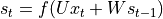 . That is, the value of the current state is the result of non-linear information combination of the previous state and the current input.
Linear transformation of the current state
through the matrix  to get the output of the current moment .
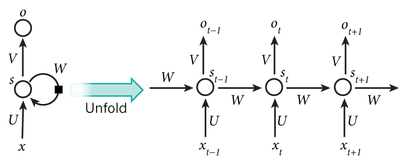
RNN working process (from http://www.wildml.com/2015/09/recurrent-neural-networks-tutorial-part-1-introduction-to-rnns )
We assume the dimension of the input vector , the state and the output vector are  , and
, and  respectively, then
  ,
,  ,
,  .
.
The above is an introduction to the most basic RNN type. In practice, some improved version of RNN are often used, such as LSTM (Long Short-Term Memory Neural Network, which solves the problem of gradient disappearance for longer sequences), GRU, etc.
Deep Reinforcement Learning (DRL)
Reinforcement learning (RL) emphasizes how to act based on the environment in order to maximize the intended benefits. With deep learning techniques combined, Deep Reinforcement Learning (DRL) is a powerful tool to solve decision tasks. AlphaGo, which has become widely known in recent years, is a typical application of deep reinforcement learning.
Note
You may want to read Introduction to Reinforcement Learning in the appendix to get some basic ideas of reinforcement learning.
Here, we use deep reinforcement learning to learn to play CartPole (inverted pendulum). The inverted pendulum is a classic problem in cybernetics. In this task, the bottom of a pole is connected to a cart through an axle, and the pole’s center of gravity is above the axle, making it an unstable system. Under the force of gravity, the pole falls down easily. We need to control the cart to move left and right on a horizontal track to keep the pole in vertical balance.
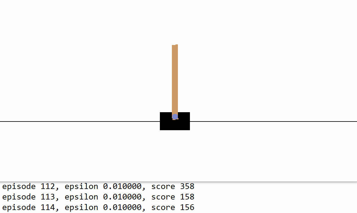
CartPole Game
We use the CartPole game environment from OpenAI’s Gym Environment Library, which can be installed using pip install gym, the installation steps and tutorials can be found in the official documentation and here. The interaction with Gym is very much like a turn-based game. We first get the initial state of the game (such as the initial angle of the pole and the position of the cart), then in each turn t, we need to choose one of the currently feasible actions and send it to Gym to execute (such as pushing the cart to the left or to the right, only one of the two actions can be chosen in each turn). After executing the action, Gym will return the next state after the action is executed and the reward value obtained in the current turn (for example, after we choose to push the cart to the left and execute, the cart position is more to the left and the angle of the pole is more to the right, Gym will return the new angle and position to us. if the pole still doesn’t go down on this round, Gym returns us a small positive reward simultaneously). This process can iterate on and on until the game ends (e.g. the pole goes down). In Python, the sample code to use Gym is as follows.
import gym

env = gym.make('CartPole-v1')   # Instantiate a game environment with the game name
state = env.reset()             # Initialize the environment, get the initial state
while True:
    env.render()                # Render the current frame and draw it to the screen.
    action = model.predict(state)   # Suppose we have a trained model that can predict what action should be performed at this time from the current state
    next_state, reward, done, info = env.step(action)   # Let the environment execute the action, get the next state of the executed action, the reward for the action, whether the game is over and additional information
    if done:                    # Exit loop if game over
        break
Now, our task is to train a model that can predict a good move based on the current state. Roughly speaking, a good move should maximize the sum of the rewards earned throughout the game, which is the goal of reinforcement learning. In the CartPole game, the goal is to make the right moves to keep the pole from falling, i.e. as many rounds of game interaction as possible. In each round, we get a small positive bonus, and the more rounds the higher the cumulative bonus value. Thus, maximizing the sum of the rewards is consistent with our ultimate goal.
The following code shows how to train the model using the Deep Q-Learning method [Mnih2013] , a classical Deep Reinforcement Learning algorithm. First, we import TensorFlow, Gym and some common libraries, and define some model hyperparameters.
import tensorflow as tf
import numpy as np
import gym
import random
from collections import deque

num_episodes = 500              # 游戏训练的总episode数量
num_exploration_episodes = 100  # 探索过程所占的episode数量
max_len_episode = 1000          # 每个episode的最大回合数
batch_size = 32                 # 批次大小
learning_rate = 1e-3            # 学习率
gamma = 1.                      # 折扣因子
initial_epsilon = 1.            # 探索起始时的探索率
final_epsilon = 0.01            # 探索终止时的探索率
We then use tf.keras.Model` to build a Q-network for fitting the Q functions in Q-Learning algorithm. Here we use a simple multilayered fully connected neural network for fitting. The network use the current state as input and outputs the Q-value for each action (2-dimensional for CartPole, i.e. pushing the cart left and right).
class QNetwork(tf.keras.Model):
    def __init__(self):
        super().__init__()
        self.dense1 = tf.keras.layers.Dense(units=24, activation=tf.nn.relu)
        self.dense2 = tf.keras.layers.Dense(units=24, activation=tf.nn.relu)
        self.dense3 = tf.keras.layers.Dense(units=2)

    def call(self, inputs):
        x = self.dense1(inputs)
        x = self.dense2(x)
        x = self.dense3(x)
        return x

    def predict(self, inputs):
        q_values = self(inputs)
Finally, we implement the Q-learning algorithm in the main program.
if __name__ == '__main__':
    env = gym.make('CartPole-v1')       # 实例化一个游戏环境,参数为游戏名称
    model = QNetwork()
    optimizer = tf.keras.optimizers.Adam(learning_rate=learning_rate)
    replay_buffer = deque(maxlen=10000) # 使用一个 deque 作为 Q Learning 的经验回放池
    epsilon = initial_epsilon
    for episode_id in range(num_episodes):
        state = env.reset()             # 初始化环境,获得初始状态
        epsilon = max(                  # 计算当前探索率
            initial_epsilon * (num_exploration_episodes - episode_id) / num_exploration_episodes,
            final_epsilon)
        for t in range(max_len_episode):
            env.render()                                # 对当前帧进行渲染,绘图到屏幕
            if random.random() < epsilon:               # epsilon-greedy 探索策略,以 epsilon 的概率选择随机动作
                action = env.action_space.sample()      # 选择随机动作(探索)
            else:
                action = model.predict(np.expand_dims(state, axis=0)).numpy()   # 选择模型计算出的 Q Value 最大的动作
                action = action[0]

            # 让环境执行动作,获得执行完动作的下一个状态,动作的奖励,游戏是否已结束以及额外信息
            next_state, reward, done, info = env.step(action)
            # 如果游戏Game Over,给予大的负奖励
            reward = -10. if done else reward
            # 将(state, action, reward, next_state)的四元组(外加 done 标签表示是否结束)放入经验回放池
            replay_buffer.append((state, action, reward, next_state, 1 if done else 0))
            # 更新当前 state
            state = next_state

            if done:                                    # 游戏结束则退出本轮循环,进行下一个 episode
                print("episode %4d, epsilon %.4f, score %4d" % (episode_id, epsilon, t))
                break

            if len(replay_buffer) >= batch_size:
                # 从经验回放池中随机取一个批次的四元组,并分别转换为 NumPy 数组
                batch_state, batch_action, batch_reward, batch_next_state, batch_done = \
                    map(np.array, zip(*random.sample(replay_buffer, batch_size)))

                q_value = model(batch_next_state)
                y = batch_reward + (gamma * tf.reduce_max(q_value, axis=1)) * (1 - batch_done)  # 计算 y 值
                with tf.GradientTape() as tape:
                    loss = tf.keras.losses.mean_squared_error(  # 最小化 y 和 Q-value 的距离
                        y_true=y,
                        y_pred=tf.reduce_sum(model(batch_state) * tf.one_hot(batch_action, depth=2), axis=1)
                    )
                grads = tape.gradient(loss, model.variables)
                optimizer.apply_gradients(grads_and_vars=zip(grads, model.variables))       # 计算梯度并更新参数
For different tasks (or environments), we need to design different states and adopt appropriate networks to fit the Q function depending on the characteristics of the task. For example, if we consider the classic “Block Breaker” game (Breakout-v0 in the Gym environment library), every action performed (baffle moving to the left, right, or motionless) returns an RGB image of 210 * 160 * 3 representing the current screen. In order to design a suitable state representation for this game, we have the following analysis.
The colour information of the bricks is not very important and the conversion of the image to grayscale does not affect the operation, so the colour information in the state can be removed (i.e. the image can be converted to grayscale).
Information on the movement of the ball is important. For CartPole, it is difficult for even a human being to judge the direction in which the baffle should move if only a single frame is known (so the direction in which the ball is moving is not known). Therefore, information that characterizes motion direction of the ball should be added to the state. A simple way is to stack the current frame with the previous frames to obtain a state representation of
210 * 160 * X(X being the number of stacked frames).The resolution of each frame does not need to be particularly high, as long as the position of the blocks, ball and baffle can be roughly characterized for decision-making purposes, so that the length and width of each frame can be compressed appropriately.
Considering that we need to extract features from the image information, using CNN as a network for fitting Q functions would be more appropriate. Based on the analysis, we can just replace the QNetwork model class above to a CNN-based model and make some changes for the status, then the same program can be used to play some simple video games like “Block Breaker”.
Keras Pipeline *
Until now, all the examples are using Keras’ Subclassing API and customized training loop. That is, we inherit tf.keras.Model class to build our new model, while the process of training and evaluating the model is explicitly implemented by us. This approach is flexible and similar to other popular deep learning frameworks (e.g. PyTorch and Chainer), and is the approach recommended in this handbook. In many cases, however, we just need to build a neural network with a relatively simple and typical structure (e.g., MLP and CNN in the above section) and train it using conventional means. For these scenarios, Keras also give us another simpler and more efficient built-in way to build, train and evaluate models.
Use Keras Sequential/Functional API to build models
The most typical and common neural network structure is to stack a bunch of layers in a specific order, so can we just provide a list of layers and have Keras automatically connect them head to tail to form a model? This is exactly what Keras Sequential API does. By providing a list of layers to tf.keras.models.Sequential(), we can quickly construct a tf.keras.Model model.
        model = tf.keras.models.Sequential([
            tf.keras.layers.Flatten(),
            tf.keras.layers.Dense(100, activation=tf.nn.relu),
            tf.keras.layers.Dense(10),
            tf.keras.layers.Softmax()
        ])
However, the sequential network structure is quite limited. Then Keras provides a more powerful functional API to help us build complex models, such as models with multiple inputs/outputs or where parameters are shared. This is done by using the layer as an invocable object and returning the tensor (which is consistent with the usage in the previous section). Then we can build a model by providing the input and output vectors to the inputs and outputs parameters of tf.keras.Model, as follows
        inputs = tf.keras.Input(shape=(28, 28, 1))
        x = tf.keras.layers.Flatten()(inputs)
        x = tf.keras.layers.Dense(units=100, activation=tf.nn.relu)(x)
        x = tf.keras.layers.Dense(units=10)(x)
        outputs = tf.keras.layers.Softmax()(x)
        model = tf.keras.Model(inputs=inputs, outputs=outputs)
Train and evaluate models using the compile, fit and evaluate methods of Keras
When the model has been built, the training process can be configured through the compile method of tf.keras.Model.
    model.compile(
        optimizer=tf.keras.optimizers.Adam(learning_rate=0.001),
        loss=tf.keras.losses.sparse_categorical_crossentropy,
        metrics=[tf.keras.metrics.sparse_categorical_accuracy]
    )
tf.keras.Model.compile accepts three important parameters.
oplimizer: an optimizer, can be selected from ``tf.keras.optimizers’’.loss: a loss function, can be selected from ``tf.keras.loses’’.metrics: a metric, can be selected fromtf.keras.metrics.
Then, the fit method of tf.keras.Model can be used to actually train the model.
model.fit(data_loader.train_data, data_loader.train_label, epochs=num_epochs, batch_size=batch_size)
tf.keras.model.fit accepts five important parameters.
x: training data.y: target data (labels of data).epochs: the number of iterations through training data.batch_size: the size of the batch.validation_data: validation data that can be used to monitor the performance of the model during training.
Keras supports tf.data.Dataset as data source, detailed in tf.data.
Finally, we can use tf.keras.Model.evaluate to evaluate the trained model, just by providing the test data and labels.
print(model.evaluate(data_loader.test_data, data_loader.test_label))
Custom layers, losses and metrics *
Perhaps you will also ask, what if these existing layers do not meet my requirements, and I need to define my own layers? In fact, we can inherit not only tf.keras.Model to write our own model classes, but also tf.keras.layers.Layer to write our own layers.
Custom layers
The custom layer requires inheriting the tf.keras.layers.Layer class and overriding the __init__, build and call methods, as follows.
class MyLayer(tf.keras.layers.Layer):
    def __init__(self):
        super().__init__()
        # Initialization code

    def build(self, input_shape): # input_shape is a TensorShape object that provides the shape of the input
        # this part of the code will run at the first time you call this layer
        # you can create variables here so that the the shape of the variable is adaptive to the input shape
        # If the shape of the variable can already be fully determined without the infomation of input shape
        # you can also create the variable in the constructor (__init__)
        self.variable_0 = self.add_weight(...)
        self.variable_1 = self.add_weight(...)

    def call(self, inputs):
        # Code for model call (handles inputs and returns outputs)
        return output
For example, we can implement a fully-connected layer on our own with the following code. This code creates two variables in the build method and uses the created variables in the call method.
class LinearLayer(tf.keras.layers.Layer):
    def __init__(self, units):
        super().__init__()
        self.units = units

    def build(self, input_shape):     # 这里 input_shape 是第一次运行call()时参数inputs的形状
        self.w = self.add_weight(name='w',
            shape=[input_shape[-1], self.units], initializer=tf.zeros_initializer())
        self.b = self.add_weight(name='b',
            shape=[self.units], initializer=tf.zeros_initializer())

    def call(self, inputs):
        y_pred = tf.matmul(inputs, self.w) + self.b
        return y_pred
When defining a model, we can use our custom layer LinearLayer just like other pre-defined layers in Keras.
class LinearModel(tf.keras.Model):
    def __init__(self):
        super().__init__()
        self.layer = LinearLayer(units=1)

    def call(self, inputs):
        output = self.layer(inputs)
        return output
Custom loss functions and metrics
The custom loss function needs to inherit the tf.keras.losses.Loss class and override the call method. The call method use the real value y_true and the model predicted value y_pred as input, and return the customized loss value between the model predicted value and the real value. The following example implements a mean square error loss function.
class MeanSquaredError(tf.keras.losses.Loss):
    def call(self, y_true, y_pred):
        return tf.reduce_mean(tf.square(y_pred - y_true))
The custom metrics need to inherit the tf.keras.metrics.Metric class and override the __init__, update_state and result methods. The following example re-implements a simple SparseCategoricalAccuracy metric class that we used earlier.
class SparseCategoricalAccuracy(tf.keras.metrics.Metric):
    def __init__(self):
        super().__init__()
        self.total = self.add_weight(name='total', dtype=tf.int32, initializer=tf.zeros_initializer())
        self.count = self.add_weight(name='count', dtype=tf.int32, initializer=tf.zeros_initializer())

    def update_state(self, y_true, y_pred, sample_weight=None):
        values = tf.cast(tf.equal(y_true, tf.argmax(y_pred, axis=-1, output_type=tf.int32)), tf.int32)
        self.total.assign_add(tf.shape(y_true)[0])
        self.count.assign_add(tf.reduce_sum(values))

    def result(self):
        return self.count / self.total
- LeCun1998
LeCun, L. Bottou, Y. Bengio, and P. Haffner. “Gradient-based learning applied to document recognition.” Proceedings of the IEEE, 86(11):2278-2324, November 1998. http://yann.lecun.com/exdb/mnist/
- Graves2013
Graves, Alex. “Generating Sequences With Recurrent Neural Networks.” ArXiv:1308.0850 [Cs], August 4, 2013. http://arxiv.org/abs/1308.0850.
- Mnih2013
Mnih, Volodymyr, Koray Kavukcuoglu, David Silver, Alex Graves, Ioannis Antonoglou, Daan Wierstra, and Martin Riedmiller. “Playing Atari with Deep Reinforcement Learning.” ArXiv:1312.5602 [Cs], December 19, 2013. http://arxiv.org/abs/1312.5602.