Common Modules in TensorFlow

Prerequisite

• Python serialization module Pickle (not required)

• Python’s special function parameter **kwargs (not required)

• Python iterator

Variable saving and restore: tf.train.Checkpoint

Warning

Checkpoint only saves the parameters (variables) of the model, not the calculation process of the model, so it is generally used to recover previously trained model parameters when the model source code is available. If you need to export the model (and run it without source code), please refer to SavedModel in the “Deployment” section.

In many scenarios, we want to save the trained parameters (variables) after the model training is complete. By loading models and parameters elsewhere where they need to be used, you can get trained models directly. Probably the first thing that comes to mind is to use pickle in Python to serialize model.variables. Unfortunately, TensorFlow’s variable type ResourceVariable cannot be serialized.

The good thing is that, TensorFlow provides a powerful variable save and restore class, tf.train.Checkpoint, which can save and restore all objects in TensorFlow that contain Checkpointable State using its save() and restore() methods. Specifically, TensorFlow instances including tf.keras.optimizer, tf.Variable, tf.keras.Layer and tf.keras.Model can be saved.

Checkpoint is very easy to use, we start by declaring a Checkpoint.

checkpoint = tf.train.Checkpoint(model=model)

Here the tf.train.Checkpoint() accepts a special initialization parameter, a **kwargs. It is a series of key-value pairs. The key names can be taken by your own, and the values are the objects to be saved. For example, if we want to save an instance of model inheriting tf.keras.Model and an optimizer optimizer inheriting tf.train.Optimizer, we could write

checkpoint = tf.train.Checkpoint(myAwesomeModel=model, myAwesomeOptimizer=optimizer)

Here myAwesomeModel is an arbitrary key name we take for the model instance that we want to save. Note that we will also use this key name when recovering variables.

Next, when the model training is complete and needs to be saved, use

checkpoint.save(save_path_with_prefix)

and things are all set. save_path_with_prefix is the save directory with prefix.

Note

For example, by creating a folder named “save” in the source directory and calling checkpoint.save('./save/model.ckpt'), we can find three files named checkpoint, model.ckpt-1.index, model.ckpt-1.data-00000-of-00001 in the save directory, and these files record variable information. The checkpoint.save() method can be run several times, and each run will result in a .index file and a .data file, with serial numbers added in sequence.

When the variable values of a previously saved instance needs to be reloaded elsewhere, a checkpoint needs to be instantiated again, while keeping the key names consistent. Then call the checkpoint’s restore method like this

model_to_be_restored = MyModel()                                        # the same class of model that need to be restored
checkpoint = tf.train.Checkpoint(myAwesomeModel=model_to_be_restored)   # keep the key name to be "myAwesomeModel"
checkpoint.restore(save_path_with_prefix_and_index)

The model variables can then be recovered. save_path_with_prefix_and_index is the directory + prefix + number of the previously saved file. For example, calling checkpoint.store('./save/model.ckpt-1') will load a file with the prefix model.ckpt and a serial number of 1.

When multiple files are saved, we often want to load the most recent one. You can use tf.train.latest_checkpoint(save_path) to get the file name of the last checkpoint in the directory. For example, if there are 10 saved files in the save directory from model.ckpt-1.index to model.ckpt-10.index, tf.train.most_checkpoint('./save') will return ./save/model.ckpt-10.

In general, a typical code framework for saving and restoring variables is as follows

# train.py: model training stage

model = MyModel()
# Instantiate the Checkpoint, specify the model instance to be saved
# (you can also add the optimizer if you want to save it)
checkpoint = tf.train.Checkpoint(myModel=model)
# ... (model training code)
# Save the variable values to a file when the training is finished
# (you can also save them regularly during the training)
checkpoint.save('./save/model.ckpt')

# test.py: model inference stage

model = MyModel()
# Instantiate the Checkpoint and specify the instance to be recovered.
checkpoint = tf.train.Checkpoint(myModel=model)
# recover the variable values of the model instance
checkpoint.restore(tf.train.latest_checkpoint('./save'))
# ... (model inference code)

Note

tf.train.Checkpoint is stronger than the tf.train.Saver commonly used in TensorFlow 1.X, in that it supports “delayed” recovery of variables in eager execution mode. Specifically, when checkpoint.store() is called, but the variable in the model has not been created, Checkpoint can wait until the variable is created to recover the value. In eager execution mode, the initialization of the layers in the model and the creation of variables is done when the model is first called (the advantage is that the variable shape can be determined automatically based on the input tensor shape, without having to be specified manually). This means that when the model has just been instantiated, there is not even a single variable in it, and it is bound to raise error to recover the variable values if we keep the same way as before. For example, you can try calling the save_weight() method of tf.keras.Model in train.py to save the parameters of the model, and call the load_weight() method immediately after instantiating the model in test.py. You will get an error. Only if you call the model once can you recover the variable values via load_weight(). If you use tf.train.Checkpoint, you do not need to worry about this. In addition, tf.train.Checkpoint also supports graph execution mode.

Finally, we provide an example of saving and restore of model variables, based on the multi-layer perceptron in the previous chapter

import tensorflow as tf
import numpy as np
import argparse
from zh.model.mnist.mlp import MLP
from zh.model.utils import MNISTLoader

parser = argparse.ArgumentParser(description='Process some integers.')
parser.add_argument('--mode', default='train', help='train or test')
parser.add_argument('--num_epochs', default=1)
parser.add_argument('--batch_size', default=50)
parser.add_argument('--learning_rate', default=0.001)
args = parser.parse_args()
data_loader = MNISTLoader()


def train():
    model = MLP()
    optimizer = tf.keras.optimizers.Adam(learning_rate=args.learning_rate)
    num_batches = int(data_loader.num_train_data // args.batch_size * args.num_epochs)
    checkpoint = tf.train.Checkpoint(myAwesomeModel=model)      # 实例化Checkpoint，设置保存对象为model
    for batch_index in range(1, num_batches+1):                 
        X, y = data_loader.get_batch(args.batch_size)
        with tf.GradientTape() as tape:
            y_pred = model(X)
            loss = tf.keras.losses.sparse_categorical_crossentropy(y_true=y, y_pred=y_pred)
            loss = tf.reduce_mean(loss)
            print("batch %d: loss %f" % (batch_index, loss.numpy()))
        grads = tape.gradient(loss, model.variables)
        optimizer.apply_gradients(grads_and_vars=zip(grads, model.variables))
        if batch_index % 100 == 0:                              # 每隔100个Batch保存一次
            path = checkpoint.save('./save/model.ckpt')         # 保存模型参数到文件
            print("model saved to %s" % path)


def test():
    model_to_be_restored = MLP()
    # 实例化Checkpoint，设置恢复对象为新建立的模型model_to_be_restored
    checkpoint = tf.train.Checkpoint(myAwesomeModel=model_to_be_restored)      
    checkpoint.restore(tf.train.latest_checkpoint('./save'))    # 从文件恢复模型参数
    y_pred = np.argmax(model_to_be_restored.predict(data_loader.test_data), axis=-1)
    print("test accuracy: %f" % (sum(y_pred == data_loader.test_label) / data_loader.num_test_data))


if __name__ == '__main__':
    if args.mode == 'train':
        train()
    if args.mode == 'test':
        test()

After creating the save folder in the code directory and running the training code, the save folder will hold model variable data that is saved every 100 batches. Adding --mode=test to the command line argument and running the code again, the model will be restored using the last saved variable values. Then we can directly obtain an accuracy rate of about 95% on test set.

Use tf.train.CheckpointManager to delete old Checkpoints and customize file numbers

During the training of the model, sometimes we’ll have the following needs

• After a long training period, the program will save a large number of Checkpoints, but we only want to keep the last few Checkpoints.

• Checkpoint is numbered by default from 1, accruing 1 at a time, but we may want to use another numbering method (e.g. using the current number of batch as the file number).

We can use TensorFlow’s tf.train.CheckpointManager to satisfy these needs. After instantiating a Checkpoint, we instantiate a CheckpointManager

checkpoint = tf.train.Checkpoint(model=model)
manager = tf.train.CheckpointManager(checkpoint, directory='./save', checkpoint_name='model.ckpt', max_to_keep=k)

Here, the directory parameter is the path to the saved file, checkpoint_name is the file name prefix (or ckpt by default if not provided), and max_to_keep is the number of retained checkpoints.

When we need to save the model, we can use manager.save() directly. If we wish to assign our own number to the saved Checkpoint, we can add the checkpoint_number parameter to manager.save() like manager.save(checkpoint_number=100).

The following code provides an example of using CheckpointManager to keep only the last three Checkpoint files and to use the number of the batch as the file number for the Checkpoint.

import tensorflow as tf
import numpy as np
import argparse
from zh.model.mnist.mlp import MLP
from zh.model.utils import MNISTLoader

parser = argparse.ArgumentParser(description='Process some integers.')
parser.add_argument('--mode', default='train', help='train or test')
parser.add_argument('--num_epochs', default=1)
parser.add_argument('--batch_size', default=50)
parser.add_argument('--learning_rate', default=0.001)
args = parser.parse_args()
data_loader = MNISTLoader()


def train():
    model = MLP()
    optimizer = tf.keras.optimizers.Adam(learning_rate=args.learning_rate)
    num_batches = int(data_loader.num_train_data // args.batch_size * args.num_epochs)
    checkpoint = tf.train.Checkpoint(myAwesomeModel=model)      
    # 使用tf.train.CheckpointManager管理Checkpoint
    manager = tf.train.CheckpointManager(checkpoint, directory='./save', max_to_keep=3)
    for batch_index in range(1, num_batches):
        X, y = data_loader.get_batch(args.batch_size)
        with tf.GradientTape() as tape:
            y_pred = model(X)
            loss = tf.keras.losses.sparse_categorical_crossentropy(y_true=y, y_pred=y_pred)
            loss = tf.reduce_mean(loss)
            print("batch %d: loss %f" % (batch_index, loss.numpy()))
        grads = tape.gradient(loss, model.variables)
        optimizer.apply_gradients(grads_and_vars=zip(grads, model.variables))
        if batch_index % 100 == 0:
            # 使用CheckpointManager保存模型参数到文件并自定义编号
            path = manager.save(checkpoint_number=batch_index)         
            print("model saved to %s" % path)


def test():
    model_to_be_restored = MLP()
    checkpoint = tf.train.Checkpoint(myAwesomeModel=model_to_be_restored)      
    checkpoint.restore(tf.train.latest_checkpoint('./save'))
    y_pred = np.argmax(model_to_be_restored.predict(data_loader.test_data), axis=-1)
    print("test accuracy: %f" % (sum(y_pred == data_loader.test_label) / data_loader.num_test_data))


if __name__ == '__main__':
    if args.mode == 'train':
        train()
    if args.mode == 'test':
        test()

Visualization of training process: TensorBoard

Sometimes you may want to see how indicators change during model training (e.g. the loss value). Although it can be viewed via command line output, it seems not intuitive enough. And TensorBoard is a tool that can help us visualize the training process.

Real-time monitoring of indicator change

To use TensorBoard, first create a folder (e.g. ./tensorboard) in the code directory to hold the TensorBoard log files, then instantiate a logger as follows

summary_writer = tf.summary.create_file_writer('./tensorboard')     # the parameter is the log folder we created

Next, when it is necessary to record the indicators during training, the value of the indicators during training at STEP can be logged by specifying the logger with the WITH statement and running tf.summary.scalar(name, tensor, step=batch_index) for the indicator (usually scalar) to be logged. The STEP parameters here can be set according to your own needs and can generally be set to the index of batch in the current training process. The overall framework is as follows.

summary_writer = tf.summary.create_file_writer('./tensorboard')
# start model training
for batch_index in range(num_batches):
    # ... (training code, use variable "loss" to store current loss value)
    with summary_writer.as_default():                               # the logger to be used
        tf.summary.scalar("loss", loss, step=batch_index)
        tf.summary.scalar("MyScalar", my_scalar, step=batch_index)  # you can also add other indicators below

For every run of tf.summary.scalar(), the logger writes a log to the log file. In addition to the simplest scalar (scalar), TensorBoard can also visualize other types of data like image and audio, as detailed in the TensorBoard documentation.

When we want to visualize the training process, open the terminal in the code directory (and go to TensorFlow’s conda environment if needed) and run:

tensorboard --logdir=./tensorboard

The visual interface of the TensorBoard can then be accessed by using a browser to access the URL output from the command line program (usually http://name-of-your-computer:6006), as shown in the following figure.

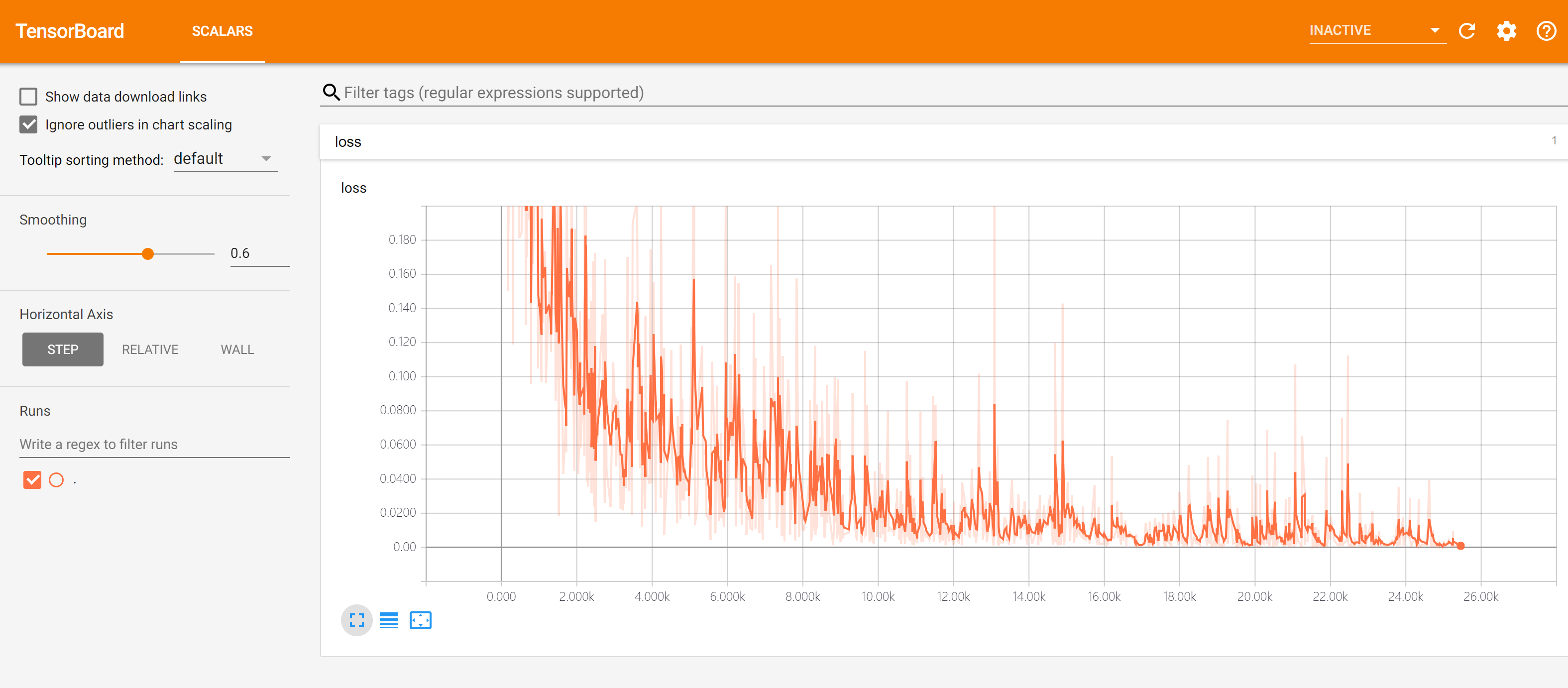
By default, TensorBoard updates data every 30 seconds. But you can also refresh manually by clicking the refresh button in the top right corner.

The following caveats apply to the use of TensorBoard.

• If retraining is required, the information in the logging folder needs to be deleted and TensorBoard need to be restarted (or you can create a new logging folder and start another TensorBoard process, with the -logdir parameter set to the newly created folder).

• Log folder path should not contain any special characters.

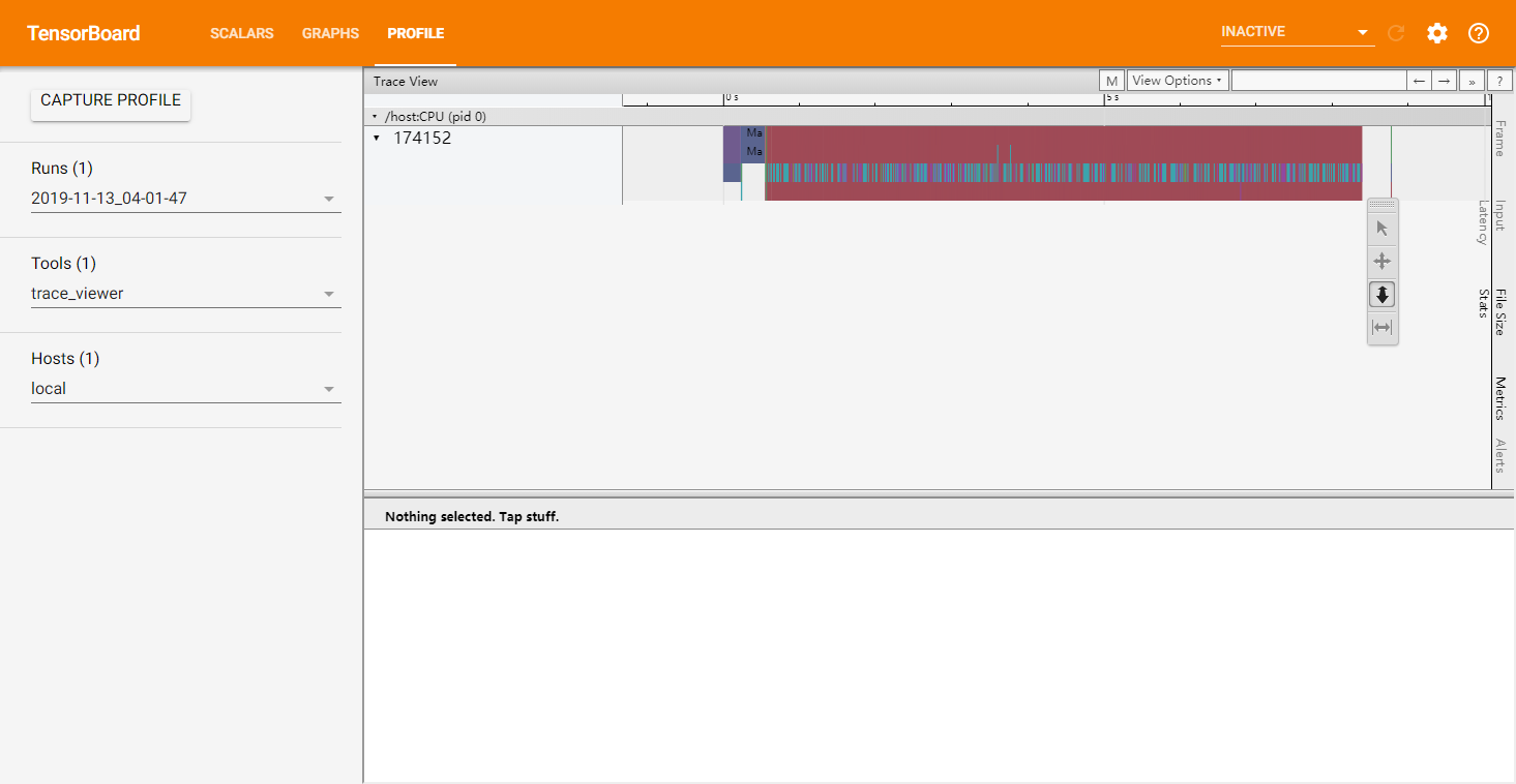
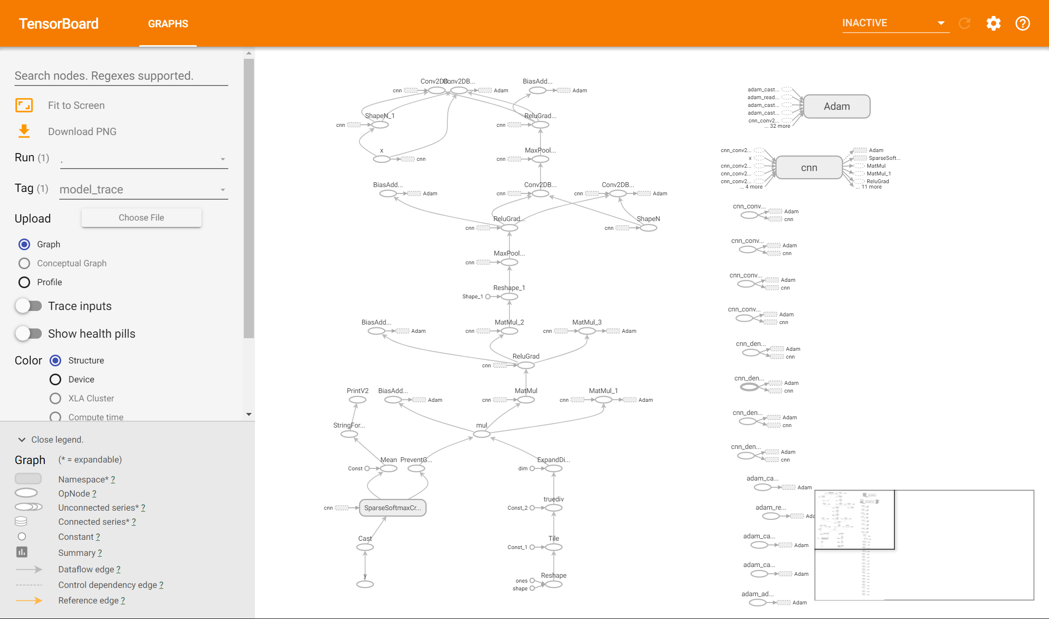
Visualize Graph and Profile Information

We can also use tf.summary.trace_on to open Trace during training, where TensorFlow records a lot of information during training, such as the structure of the dataflow graph, and the time spent on each operation. When training is complete, you can use tf.summary.trace_export to export the recorded results to a file.

tf.summary.trace_on(graph=True, profiler=True)  # Open Trace option, then the dataflow graph and profiling information can be recorded
# ... (training code)
with summary_writer.as_default():
    tf.summary.trace_export(name="model_trace", step=0, profiler_outdir=log_dir)    # Save Trace information to a file

After that, we can select “Profile” in TensorBoard to see the time spent on each operation in a timeline. If you have created a dataflow graph using tf.function, you can also click “Graph” to view the graph structure.

Example: visualize the training process of MLP

Finally, we provide an example of the TensorBoard usage based on multi-layer perceptron model in the previous chapter.

import tensorflow as tf
from zh.model.mnist.mlp import MLP
from zh.model.utils import MNISTLoader

num_batches = 1000
batch_size = 50
learning_rate = 0.001
log_dir = 'tensorboard'
model = MLP()
data_loader = MNISTLoader()
optimizer = tf.keras.optimizers.Adam(learning_rate=learning_rate)
summary_writer = tf.summary.create_file_writer(log_dir)     # 实例化记录器
tf.summary.trace_on(profiler=True)  # 开启Trace（可选）
for batch_index in range(num_batches):
    X, y = data_loader.get_batch(batch_size)
    with tf.GradientTape() as tape:
        y_pred = model(X)
        loss = tf.keras.losses.sparse_categorical_crossentropy(y_true=y, y_pred=y_pred)
        loss = tf.reduce_mean(loss)
        print("batch %d: loss %f" % (batch_index, loss.numpy()))
        with summary_writer.as_default():                           # 指定记录器
            tf.summary.scalar("loss", loss, step=batch_index)       # 将当前损失函数的值写入记录器
    grads = tape.gradient(loss, model.variables)
    optimizer.apply_gradients(grads_and_vars=zip(grads, model.variables))
with summary_writer.as_default():
    tf.summary.trace_export(name="model_trace", step=0, profiler_outdir=log_dir)    # 保存Trace信息到文件（可选）

Dataset construction and preprocessing: tf.data

In many scenarios, we want to use our own datasets to train the model. However, the process of preprocessing and reading raw data files is often cumbersome and even more labor-intensive than the design of the model. For example, in order to read a batch of image files, we may need to struggle with python’s various image processing packages (such as pillow), design our own batch generation method, and finally may not run as efficiently as expected. To this end, TensorFlow provides the tf.data module, which includes a flexible set of dataset building APIs that help us quickly and efficiently build data input pipelines, especially for large-scale scenarios.

Dataset construction

At the heart of tf.data is the tf.data.Dataset class, which provides a high-level encapsulation of the TensorFlow dataset. tf.data.Dataset consists of a series of iteratively accessible elements, each containing one or more tensor. For example, for a dataset consisting of images, each element can be an image tensor with the shape width x height x number of channels, or a tuple consisting of an image tensor and an image label tensor.

The most basic way to build tf.data.Dataset is to use tf.data.Dataset.from_tensor_slices() for small amount of data (which can fit into the memory). Specifically, if all the elements of our dataset are stacked together into a large tensor through the 0-th dimension of the tensor (e.g., the training set of the MNIST dataset in the previous section is one large tensor with shape [60000, 28, 28, 1], representing 60,000 single-channel grayscale image of size 28*28), then we provide such one or more large tensor as input, and can construct the dataset by unstack it on the 0-th dimension of the tensor. In this case, the size of the 0-th dimension is the number of data elements in the dataset. We have an example as follows

import tensorflow as tf
import numpy as np

X = tf.constant([2013, 2014, 2015, 2016, 2017])
Y = tf.constant([12000, 14000, 15000, 16500, 17500])

# 也可以使用NumPy数组，效果相同
# X = np.array([2013, 2014, 2015, 2016, 2017])
# Y = np.array([12000, 14000, 15000, 16500, 17500])

dataset = tf.data.Dataset.from_tensor_slices((X, Y))

for x, y in dataset:
    print(x.numpy(), y.numpy()) 

Output:

2013 12000
2014 14000
2015 15000
2016 16500
2017 17500

Warning

When multiple tensors are provided as input, the size of 0-th dimension of these tensors must be the same, and the multiple tensors must be spliced as tuples (i.e., using parentheses in Python).

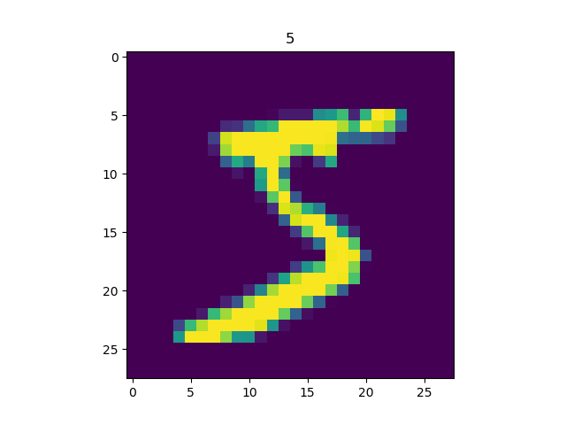
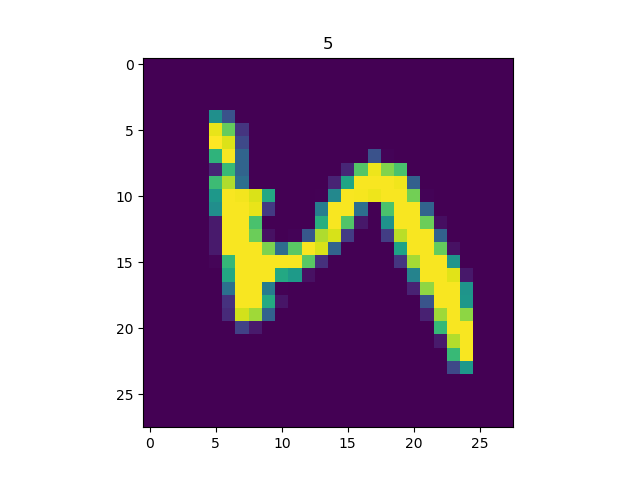
Similarly, we can load the MNIST dataset in the previous chapter.

import matplotlib.pyplot as plt 

(train_data, train_label), (_, _) = tf.keras.datasets.mnist.load_data()
train_data = np.expand_dims(train_data.astype(np.float32) / 255.0, axis=-1)      # [60000, 28, 28, 1]
mnist_dataset = tf.data.Dataset.from_tensor_slices((train_data, train_label))

for image, label in mnist_dataset:
    plt.title(label.numpy())
    plt.imshow(image.numpy()[:, :, 0])
    plt.show()

Output

Hint

TensorFlow Datasets provides an out-of-the-box collection of datasets based on tf.data.Datasets. You can view TensorFlow Datasets for the detailed usage. For example, we can load the MNIST dataset in just two lines of code:

import tensorflow_datasets as tfds
dataset = tfds.load("mnist", split=tfds.Split.TRAIN, as_supervised=True)

For extremely large datasets that cannot be fully loaded into the memory, we can first process the datasets in TFRecord format and then use tf.data.TFRocrdDataset() to load them. You can refer to the TFRecord section for details.

Dataset preprocessing

The tf.data.Dataset class provides us with a variety of dataset preprocessing methods. Some of the most commonly used methods are

• Dataset.map(f): apply the function f to each element of the dataset to obtain a new dataset (this part is often combined with tf.io to read, write and decode files and tf.image to process images).

• Dataset.shuffle(buffer_size): shuffle the dataset (set a fixed-size buffer, put the first buffer_size element in the buffer, and sample randomly from the buffer, replacing the sampled data with subsequent data).

• Dataset.batch(batch_size): batches the dataset, i.e. for each batch_size elements, using ``tf.stack()` to merge into one element on dimension 0.

In addition, there are Dataset.repeat() (repeat elements in the dataset), Dataset.reduce() (aggregation operation), Dataset.take() (interception of the first few elements of a dataset), etc. Further description can be found in the API document.

The following example is based on the MNIST data set.

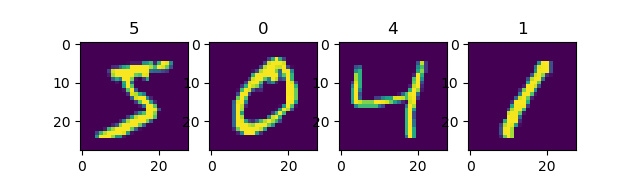
Using Dataset.map() to rotate all pictures 90 degrees.

def rot90(image, label):
    image = tf.image.rot90(image)
    return image, label

mnist_dataset = mnist_dataset.map(rot90)

for image, label in mnist_dataset:
    plt.title(label.numpy())
    plt.imshow(image.numpy()[:, :, 0])
    plt.show()

Output:

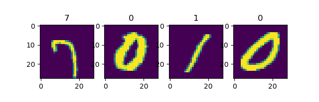
Use Dataset.batch() to divide the dataset into batches, each with a size of 4.

mnist_dataset = mnist_dataset.batch(4)

for images, labels in mnist_dataset:    # image: [4, 28, 28, 1], labels: [4]
    fig, axs = plt.subplots(1, 4)
    for i in range(4):
        axs[i].set_title(labels.numpy()[i])
        axs[i].imshow(images.numpy()[i, :, :, 0])
    plt.show()

Output:

Use Dataset.shuffle() to shuffle the dataset with the cache size set to 10000, and then set the batch.

mnist_dataset = mnist_dataset.shuffle(buffer_size=10000).batch(4)

for images, labels in mnist_dataset:
    fig, axs = plt.subplots(1, 4)
    for i in range(4):
        axs[i].set_title(labels.numpy()[i])
        axs[i].imshow(images.numpy()[i, :, :, 0])
    plt.show()

Output:

The first run

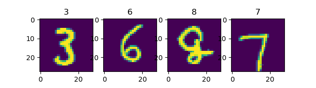
The second run

It can be seen that each time the data is randomly shuffled.

buffer_size setting of Dataset.shuffle()

As an iterator designed for large-scale data, tf.data.Dataset does not support easy access to the number of its own elements or random access to elements. Therefore, in order to shuffle the data set efficiently, some specific designed methods are needed. Dataset.shuffle() took the following approach.

• Set a buffer with fixed size buffer_size.

• At initialization, the first buffer_size element of the dataset is moved to the buffer.

• Each time an element needs to be randomly taken from the dataset, then one element is randomly sampled and taken out from the buffer (so there is an empty space in the buffer), and then one subsequent element in the dataset is taken out and put back into the empty space to maintain the size of the buffer.

Therefore, the size of the buffer needs to be set reasonably according to the characteristics of the dataset. For example.

• When buffer_size is set to 1, it is equivalent to no shuffling at all.

• When the label order of the dataset is extremely unevenly distributed (e.g., the first half labels of the dataset are 0 and the second half labels are 1 in binary classification), a small buffer size will result in all elements in a batch to have same label, thus affecting the training effect. In general, the size of the buffer can be smaller if the distribution of the dataset is more random, otherwise a larger buffer is required.

Increase the efficiency using the parallelization strategy of tf.data

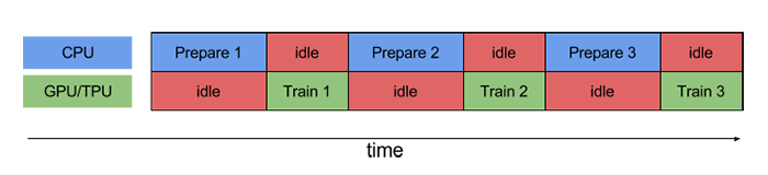
When training models, we want to make the most of computing resources and reduce CPU/GPU idle time. However, sometimes, the preparation of dataset is very time-consuming, thus we have to spend a lot of time preparing data for training before each batch of training. When we are preparing the data, the GPU can only wait for data with no load, resulting in a waste of computing resources, as shown in the following figure.

Original training process, GPU can only be idle when preparing data. Source 1 。

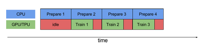
To tackle this problem, tf.data provides us with the Dataset.prefetch() method, which allows us to let the dataset prefetch several elements during training, so that the CPU can prepare data while training in the GPU, improving the efficiency of the training process, as shown below.

The usage of Dataset.prefetch() is very similar to Dataset.batch() and Dataset.shuffle() in the previous section. Continuing with the MNIST dataset example, if you want to preloaded data, you can use the following code

mnist_dataset = mnist_dataset.prefetch(buffer_size=tf.data.experimental.AUTOTUNE)

Here the parameter buffer_size can be set either manually, or set to tf.data.experimental.AUTOTUNE to let TensorFlow select the appropriate value automatically.

Similarly, Dataset.map() can also transform data elements in parallel with multiple GPU resources to increase efficiency. Take the MNIST dataset as an example. assumes that the training machine has a 2-core CPU, and we want to take full advantage of the multi-core CPU to perform a parallelized transformation of the data (e.g. the 90-degree rotation function rot90 in the previous section), we can using the following code

mnist_dataset = mnist_dataset.map(map_func=rot90, num_parallel_calls=2)

The operation process is shown in the following figure.

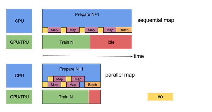
Parallelization of data conversion is achieved by setting the num_parallel_calls parameter of Dataset.map(). The top part is unparallelized and the bottom part is 2-core parallel. Source 3 。

It is also possible to set num_parallel_calls to tf.data.experimental.AUTOTUNE to allow TensorFlow to automatically select the appropriate value.

In addition to this, there are a number of ways to improve dataset processing performance, which can be found in the TensorFlow documentation. The powerful performance of the tf.data parallelization policy is demonstrated in a later example, which can be viewed here.

Fetching elements from datasets

After the data is constructed and pre-processed, we need to iterate through it to get the data for training. tf.data.Dataset is an iteratable Python object, so data can be obtained using the For loop iteratively, namely.

dataset = tf.data.Dataset.from_tensor_slices((A, B, C, ...))
for a, b, c, ... in dataset:
    # Operate on tensor a, b, c, etc., e.g. feed into model for training

You can also use ``iter()` to explicitly create a Python iterator and use ``next()` to get the next element, namely.

dataset = tf.data.Dataset.from_tensor_slices((A, B, C, ...))
it = iter(dataset)
a_0, b_0, c_0, ... = next(it)
a_1, b_1, c_1, ... = next(it)

Keras supports the use of tf.data.Dataset directly as input. When calling the fit() and evaluate() methods of tf.keras.Model, the input data x in the parameter can be specified as Dataset with all elements formatted as (input data, label data) ``. In this case, the parameter ``y (label data) can be ignored. For example, for the MNIST dataset mentioned above, the original Keras training approach is.

model.fit(x=train_data, y=train_label, epochs=num_epochs, batch_size=batch_size)

After using tf.data.Dataset, we can pass the dataset directly into Keras API.

model.fit(mnist_dataset, epochs=num_epochs)

Since the dataset have already been divided into batches by the Dataset.batch() method, we do not need to provide the size of the batch to model.fit().

Example: cats_vs_dogs image classification

The following code, using the “Cat and Dog” binary image classification task as an example, demonstrates the complete process of building, training and testing model with tf.data combined with tf.io and tf.image. The dataset can be downloaded here. The dataset should be decompressed into the data_dir directory in the code (here the default setting is C:/datasets/cats_vs_dogs, which can be modified to suit your needs).

import tensorflow as tf
import os

num_epochs = 10
batch_size = 32
learning_rate = 0.001
data_dir = 'C:/datasets/cats_vs_dogs'
train_cats_dir = data_dir + '/train/cats/'
train_dogs_dir = data_dir + '/train/dogs/'
test_cats_dir = data_dir + '/valid/cats/'
test_dogs_dir = data_dir + '/valid/dogs/'

def _decode_and_resize(filename, label):
    image_string = tf.io.read_file(filename)            # 读取原始文件
    image_decoded = tf.image.decode_jpeg(image_string)  # 解码JPEG图片
    image_resized = tf.image.resize(image_decoded, [256, 256]) / 255.0
    return image_resized, label

if __name__ == '__main__':
    # 构建训练数据集
    train_cat_filenames = tf.constant([train_cats_dir + filename for filename in os.listdir(train_cats_dir)])
    train_dog_filenames = tf.constant([train_dogs_dir + filename for filename in os.listdir(train_dogs_dir)])
    train_filenames = tf.concat([train_cat_filenames, train_dog_filenames], axis=-1)
    train_labels = tf.concat([
        tf.zeros(train_cat_filenames.shape, dtype=tf.int32), 
        tf.ones(train_dog_filenames.shape, dtype=tf.int32)], 
        axis=-1)

    train_dataset = tf.data.Dataset.from_tensor_slices((train_filenames, train_labels))
    train_dataset = train_dataset.map(
        map_func=_decode_and_resize, 
        num_parallel_calls=tf.data.experimental.AUTOTUNE)
    # 取出前buffer_size个数据放入buffer，并从其中随机采样，采样后的数据用后续数据替换
    train_dataset = train_dataset.shuffle(buffer_size=23000)    
    train_dataset = train_dataset.batch(batch_size)
    train_dataset = train_dataset.prefetch(tf.data.experimental.AUTOTUNE)

    model = tf.keras.Sequential([
        tf.keras.layers.Conv2D(32, 3, activation='relu', input_shape=(256, 256, 3)),
        tf.keras.layers.MaxPooling2D(),
        tf.keras.layers.Conv2D(32, 5, activation='relu'),
        tf.keras.layers.MaxPooling2D(),
        tf.keras.layers.Flatten(),
        tf.keras.layers.Dense(64, activation='relu'),
        tf.keras.layers.Dense(2, activation='softmax')
    ])

    model.compile(
        optimizer=tf.keras.optimizers.Adam(learning_rate=learning_rate),
        loss=tf.keras.losses.sparse_categorical_crossentropy,
        metrics=[tf.keras.metrics.sparse_categorical_accuracy]
    )

    model.fit(train_dataset, epochs=num_epochs)

Use the following code to test the model

    # 构建测试数据集
    test_cat_filenames = tf.constant([test_cats_dir + filename for filename in os.listdir(test_cats_dir)])
    test_dog_filenames = tf.constant([test_dogs_dir + filename for filename in os.listdir(test_dogs_dir)])
    test_filenames = tf.concat([test_cat_filenames, test_dog_filenames], axis=-1)
    test_labels = tf.concat([
        tf.zeros(test_cat_filenames.shape, dtype=tf.int32), 
        tf.ones(test_dog_filenames.shape, dtype=tf.int32)], 
        axis=-1)

    test_dataset = tf.data.Dataset.from_tensor_slices((test_filenames, test_labels))
    test_dataset = test_dataset.map(_decode_and_resize)
    test_dataset = test_dataset.batch(batch_size)

    print(model.metrics_names)
    print(model.evaluate(test_dataset))

By performing performance tests on the above examples, we can feel the powerful parallelization performance of tf.data. Through the use of prefetch() and the addition of the num_parallel_calls parameter to the map() process, the model training time can be reduced to half or even less than before. The test results are as follows.

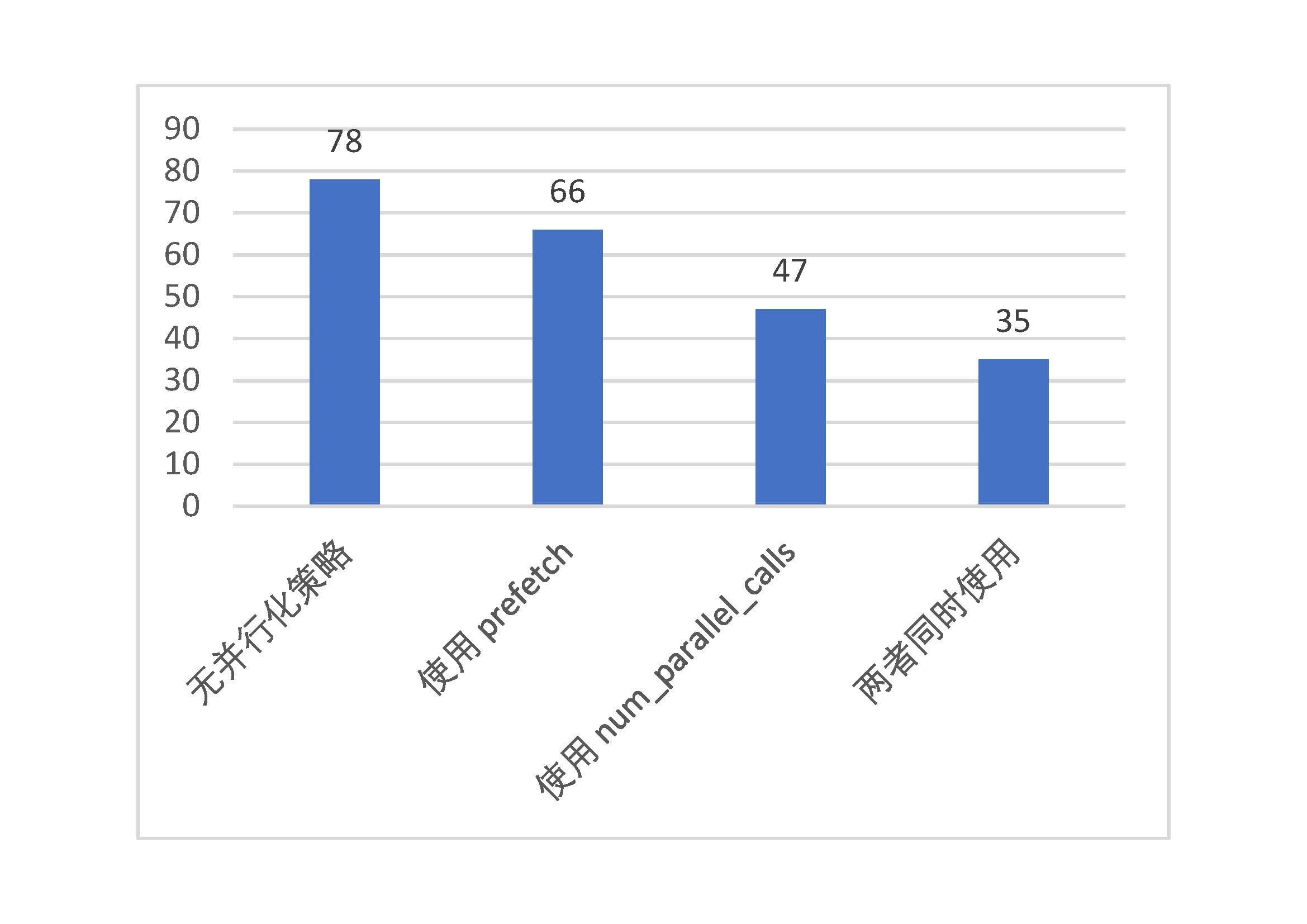
Parallelization performance test for tf.data (vertical axis is time taken per epoch, in seconds)

TFRecord: Dataset format of TensorFlow

TFRecord is the dataset storage format in TensorFlow. Once we have organized the datasets into TFRecord format, TensorFlow can read and process them efficiently, helping us to train large-scale models more efficiently.

TFRecord can be understood as a file consisting of a series of serialized tf.train.Sample elements, each tf.train.Sample consisting of a dict of several tf.train.Feature. The form is as follows.

# dataset.tfrecords
[
    {   # example 1 (tf.train.Example)
        'feature_1': tf.train.Feature,
        ...
        'feature_k': tf.train.Feature
    },
    ...
    {   # example N (tf.train.Example)
        'feature_1': tf.train.Feature,
        ...
        'feature_k': tf.train.Feature
    }
]

In order to organize the various datasets into TFRecord format, we can do the following steps for each element of the dataset.

• Read the data element into memory.

• Convert the element to tf.train.example objects (each tf.train.example consists of several tf.train.Feature, so a dictionary of Feature needs to be created first).

• Serialize the tf.train.Sample` object as a string and write it to a TFRecord file with a predefined tf.io.TFRecordWriter.

To read the TFRecord data, follow these steps.

• Obtain a tf.data.Dataset instance by reading the original TFRecord file (notice that the tf.train.Sample object in the file has not been deserialized).

• Deserialize the tf.train.Sample string by tf.io.parse_single_example function for each serialized tf.train.Sample string in the dataset through the Dataset.map method.

In the following part, we show a code example to convert the training set of the cats_vs_dogs dataset into a TFRecord file and load this file.

Convert the dataset into a TFRecord file

First, similar to the previous section, we download the dataset and extract it to data_dir. We also initialize the list of image filenames and tags for the dataset.

import tensorflow as tf
import os

data_dir = 'C:/datasets/cats_vs_dogs'
train_cats_dir = data_dir + '/train/cats/'
train_dogs_dir = data_dir + '/train/dogs/'
tfrecord_file = data_dir + '/train/train.tfrecords'

train_cat_filenames = [train_cats_dir + filename for filename in os.listdir(train_cats_dir)]
train_dog_filenames = [train_dogs_dir + filename for filename in os.listdir(train_dogs_dir)]
train_filenames = train_cat_filenames + train_dog_filenames
train_labels = [0] * len(train_cat_filenames) + [1] * len(train_dog_filenames)  # 将 cat 类的标签设为0，dog 类的标签设为1

Then, through the following code, we iteratively read each image, build the tf.train.Feature dictionary and the tf.train.Sample object, serialize it and write it to the TFRecord file.

with tf.io.TFRecordWriter(tfrecord_file) as writer:
    for filename, label in zip(train_filenames, train_labels):
        image = open(filename, 'rb').read()     # 读取数据集图片到内存，image 为一个 Byte 类型的字符串
        feature = {                             # 建立 tf.train.Feature 字典
            'image': tf.train.Feature(bytes_list=tf.train.BytesList(value=[image])),  # 图片是一个 Bytes 对象
            'label': tf.train.Feature(int64_list=tf.train.Int64List(value=[label]))   # 标签是一个 Int 对象
        }
        example = tf.train.Example(features=tf.train.Features(feature=feature)) # 通过字典建立 Example
        writer.write(example.SerializeToString())   # 将Example序列化并写入 TFRecord 文件

It is worth noting that tf.train.Feature supports three data formats.

• tf.train.BytesList: string or binary files (e.g. image). Use bytes_list parameter to pass through a tf.train.BytesList object initialized by an array of strings or bytes.

• tf.train.FloatList : float or double numbers. Use float_list parameter to pass through a tf.train.FloatList object initialized by a float or double array.

• tf.train.Int64List : integers. Use int64_list parameter to pass through a tf.train.Int64List object initialized by an array of integers.

If you want to feed in only one element rather than an array, you can pass in an array with only one element.

With the code above, we can get a file sized around 500MB named train.tfrecords.

Read the TFRecord file

We can read the file train.tfrecords created in the previous section, and decode each serialized tf.train.Example object with Dataset.map and tf.io.parse_single_example .

raw_dataset = tf.data.TFRecordDataset(tfrecord_file)    # 读取 TFRecord 文件

feature_description = { # 定义Feature结构，告诉解码器每个Feature的类型是什么
    'image': tf.io.FixedLenFeature([], tf.string),
    'label': tf.io.FixedLenFeature([], tf.int64),
}

def _parse_example(example_string): # 将 TFRecord 文件中的每一个序列化的 tf.train.Example 解码
    feature_dict = tf.io.parse_single_example(example_string, feature_description)
    feature_dict['image'] = tf.io.decode_jpeg(feature_dict['image'])    # 解码JPEG图片
    return feature_dict['image'], feature_dict['label']

dataset = raw_dataset.map(_parse_example)

The feature_description is like a “description file” of a dataset, informing the tf.io.parse_single_example function the properties of each tf.train.sample element, through a dictionary of key-value pairs. The properties contain which features are available for each tf.train.sample element, and the type, shape, and other properties of those features. The three input parameters of tf.io.FixedLenFeatures: shape, dtype and default_value (optional) are the shape, type and default values for each Feature. Here our data items are single values or strings, so shape` is an empty array.

After running the above code, we get a dataset instance dataset, which is already a tf.data.Dataset instance that can be used for training! We output an element from this dataset to validate the code

import matplotlib.pyplot as plt 

for image, label in dataset:
    plt.title('cat' if label == 0 else 'dog')
    plt.imshow(image.numpy())
    plt.show()

Output:

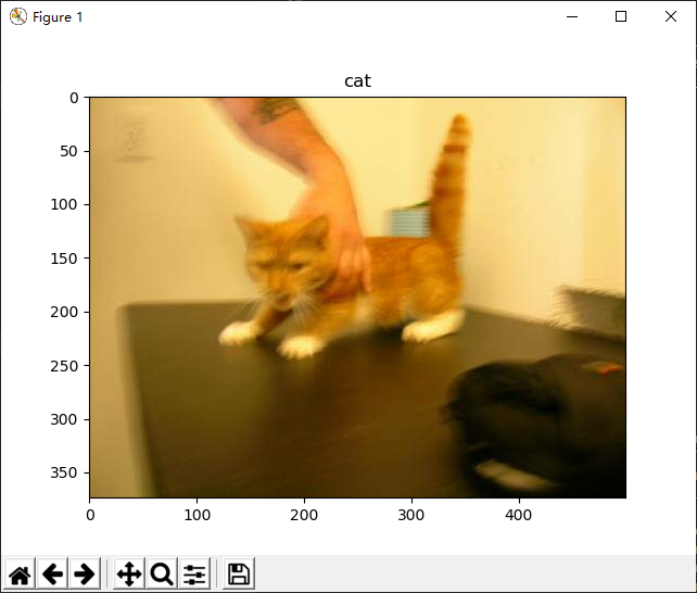
It can be seen that the images and labels are displayed correctly, and the data set is constructed successfully.

Graph execution mode: @tf.function *

While the default Eager Execution mode gives us flexibility and ease of debugging, in some scenarios, we still want to use the Graph Execution mode (default in in TensorFlow 1.X) to transform the model into an efficient TensorFlow graph model, especially when we want high performance or to deploy models. Therefore, TensorFlow 2 provides us with the tf.function module, which, in conjunction with the AutoGraph mechanism, makes it easy to run the model in graph execution mode by simply adding a @tf.function` decorator.

Basic usage of tf.function

In TensorFlow 2, it is recommended to use tf.function (instead of tf.Session in 1.X) to implement the graph execution, so that you can convert the model to an easy-to-deploy, high-performance TensorFlow graph model. To use tf.function, you can just simply encapsulate the code within a function, and decorate the function with @tf.function decorator, as shown in the example below. For an in-depth discussion of the graph execution mode, see the appendix .

Warning

Not all functions can be decorated by @tf.function! @tf.function uses static compilation to convert the code within the function into a dataflow graph, so there are restrictions on the statements that can be used within the function (only a subset of the Python language is supported), and the operations within the function need to be able to act as a node in the computational graph. It is recommended to use only native TensorFlow operations within the function, not to use overly complex Python statements, and only include TensorFlow tensors or NumPy arrays in the function arguments. In conclusion, it will be better to build the function according to the idea of a dataflow graph. @tf.function just gives you a more convenient way to write computational graphs, not a “silver bullet” that will accelerate any function. Details are available at AutoGraph Capabilities and Limitations. You can read this section together with the appendix for better understanding.

import tensorflow as tf
import time
from zh.model.mnist.cnn import CNN
from zh.model.utils import MNISTLoader

num_batches = 1000
batch_size = 50
learning_rate = 0.001
data_loader = MNISTLoader()
model = CNN()
optimizer = tf.keras.optimizers.Adam(learning_rate=learning_rate)

@tf.function
def train_one_step(X, y):    
    with tf.GradientTape() as tape:
        y_pred = model(X)
        loss = tf.keras.losses.sparse_categorical_crossentropy(y_true=y, y_pred=y_pred)
        loss = tf.reduce_mean(loss)
        # 注意这里使用了TensorFlow内置的tf.print()。@tf.function不支持Python内置的print方法
        tf.print("loss", loss)
    grads = tape.gradient(loss, model.variables)    
    optimizer.apply_gradients(grads_and_vars=zip(grads, model.variables))

start_time = time.time()
for batch_index in range(num_batches):
    X, y = data_loader.get_batch(batch_size)
    train_one_step(X, y)
end_time = time.time()
print(end_time - start_time)

With 400 batches, the program took 35.5 seconds with @tf.function and 43.8 seconds without @tf.function''. It can be seen that ``@tf.function brought some performance improvements. In general, @tf.function brings greater performance boost when the model is composed of many small operations. But if the model does not have much operations while each operation is time-consuming, the performance gains from @tf.function will not be significant.

Internal mechanism of tf.function

When the function decorated by @tf.function is called for the first time, the following is done.

• In an environment where the eager execution mode is off, the code within the function runs sequentially. That is, each TensorFlow operation API simply defines the computation node (OpNode) in a dataflow graph, and does not perform any substantive computation. This is consistent with the graph execution mode of TensorFlow 1.X.

• Use AutoGraph to convert Python control flow statements to corresponding computation nodes in the TensorFlow datagraph graph (e.g. while and for statements to tf.while, if statements to tf.cond).

• Based on the above two steps, create a dataflow graph representation of the code within the function (the graph will also automatically include some tf.control_dependencies nodes in order to ensure the computational order of the graph).

• Run this calculation once.

• Cache the built dataflow graph to a hash table. The hash key based on the name of the function and the type of function argument

When a function is called again after being decorated by @tf.function, TensorFlow will first calculate the hash key based on the function name and the type of function argument. If the corresponding dataflow graph is already in the hash table, then use the cached dataflow graph directly, otherwise recreate the dataflow graph by following the steps above.

Hint

For developers familiar with TensorFlow 1.X who want to obtain the dataflow graphs generated by tf.function directly for further processing and debugging, you can use the get_concrete_function` method of the decorated function. The method accepts the same arguments as the decorated function. For example, in order to obtain the graph generated by the function train_one_step modified by @tf.function in the previous section, the following code can be used.

graph = train_one_step.get_concrete_function(X, y)

in which the graph is an tf.Graph object.

The following is a quiz:

import tensorflow as tf
import numpy as np

@tf.function
def f(x):
    print("The function is running in Python")
    tf.print(x)

a = tf.constant(1, dtype=tf.int32)
f(a)
b = tf.constant(2, dtype=tf.int32)
f(b)
b_ = np.array(2, dtype=np.int32)
f(b_)
c = tf.constant(0.1, dtype=tf.float32)
f(c)
d = tf.constant(0.2, dtype=tf.float32)
f(d)

What is the result of this procedure above?

Answer:

The function is running in Python
1
2
2
The function is running in Python
0.1
0.2

When calculating f(a), TensorFlow does the following, since it is the first time this function is called.

• The code within the function is run through in turn (hence it output the text “The function is running in Python”).

• A dataflow graph was constructed, and then that graph was run once (thus outputting number “1”). Here tf.print(x) can be used as a node of the dataflow graph, but Python’s built-in print cannot be converted to a node of the dataflow graph. Therefore, only the operation tf.print(x) is included in the calculation graph.

• The graph is cached in a hash table (the constructed graph is reused if it is followed by a tensor input of type tf.int32 with an empty shape).

When calculating f(b), since b has the same type as a, TensorFlow reuses the previously constructed dataflow graph and runs (thus outputting number “2”). Here the text output code on the first line of the function is not run because the code in the function is not really run line by line. When calculating f(b_), TensorFlow automatically converts the numpy data structure to a tensor in TensorFlow, so it can still reuse the previously constructed graph.

When calculating f(c), although the tensor c has the same shape as a, b, but the type is tf.float32 instead. For this case, TensorFlow re-runs the code in the function (thus outputting the text again) and creates a dataflow graph with input of type tf.float32.

When calculating f(d), since d and c are of the same type, TensorFlow reuse the dataflow graph and similarly does not output text.

The treatment of Python’s built-in integer and floating-point types by @tf.function is shown by the following example.

f(d)
f(1)
f(2)
f(1)
f(0.1)
f(0.2)
f(0.1)

The result is:

The function is running in Python
1
The function is running in Python
2
1
The function is running in Python
0.1
The function is running in Python
0.2
0.1

In short, for Python’s built-in integer and floating-point types, @tf.function will only reuse a previously created graph when the values are exactly the same, and will not automatically convert Python’s built-in integers or floating-point numbers into tensors. Therefore, extra care needs to be taken if you need to contain Python’s built-in integers or floating-point numbers in function arguments. In general, Python built-in types should only be used as parameters for functions decorated by @tf.function on a few occasions, such as specifying hyperparameters.

The next quiz:

import tensorflow as tf

a = tf.Variable(0.0)

@tf.function
def g():
    a.assign(a + 1.0)
    return a

print(g())
print(g())
print(g())

The output is:

tf.Tensor(1.0, shape=(), dtype=float32)
tf.Tensor(2.0, shape=(), dtype=float32)
tf.Tensor(3.0, shape=(), dtype=float32)

As in the other examples in this handbook, you can call tf.Variable, tf.keras.optimizers, tf.keras.Model and other classes containing variables in functions decorated by @tf.function. Once called, these class instances are provided to the function as implicit arguments. When the values within these instance are modified inside the function, the modification is also valid outside the function.

AutoGraph: Converting Python control flows into TensorFlow graphs

As mentioned earlier, @tf.function uses a mechanism called “AutoGraph” to convert the Python control flow statement in the function to the corresponding node in the TensorFlow dataflow graph. Here is an example of using the low-level API of tf.autograph, tf.autograph.to_code, to convert the function square_if_positive to a TensorFlow dataflow graph.

import tensorflow as tf

@tf.function
def square_if_positive(x):
    if x > 0:
        x = x * x
    else:
        x = 0
    return x

a = tf.constant(1)
b = tf.constant(-1)
print(square_if_positive(a), square_if_positive(b))
print(tf.autograph.to_code(square_if_positive.python_function))

Output:

tf.Tensor(1, shape=(), dtype=int32) tf.Tensor(0, shape=(), dtype=int32)
def tf__square_if_positive(x):
    do_return = False
    retval_ = ag__.UndefinedReturnValue()
    cond = x > 0

    def get_state():
        return ()

    def set_state(_):
        pass

    def if_true():
        x_1, = x,
        x_1 = x_1 * x_1
        return x_1

    def if_false():
        x = 0
        return x
    x = ag__.if_stmt(cond, if_true, if_false, get_state, set_state)
    do_return = True
    retval_ = x
    cond_1 = ag__.is_undefined_return(retval_)

    def get_state_1():
        return ()

    def set_state_1(_):
        pass

    def if_true_1():
        retval_ = None
        return retval_

    def if_false_1():
        return retval_
    retval_ = ag__.if_stmt(cond_1, if_true_1, if_false_1, get_state_1, set_state_1)
    return retval_

We note that the Python control flow in the original function if... else... are automatically compiled to x = ag__.if_stmt(cond, if_true, if_false, get_state, set_state) which is based on dataflow graph. AutoGraph serves as a compiler-like function that helps us easily build dataflow graphs with conditions/loops using a more natural Python control flow, without having to build them manually using TensorFlow’s API.

Using traditional tf.Session

It is okay if you still want to use the API in TensorFlow 1.X to build dataflow graph. TensorFlow 2 provides the tf.compat.v1 module to support the TensorFlow 1.X API, and Keras model is compatible with both the eager execution and graph execution modes (with a little care when writing the model). Note that in graph execution mode, model(input_tensor) only needs to be run once to build the graph.

For example, the MLP or CNN model created in the previous chapter can also be trained on the MNIST dataset with the following code.

    optimizer = tf.compat.v1.train.AdamOptimizer(learning_rate=learning_rate)
    num_batches = int(data_loader.num_train_data // batch_size * num_epochs)
    # 建立计算图
    X_placeholder = tf.compat.v1.placeholder(name='X', shape=[None, 28, 28, 1], dtype=tf.float32)
    y_placeholder = tf.compat.v1.placeholder(name='y', shape=[None], dtype=tf.int32)
    y_pred = model(X_placeholder)
    loss = tf.keras.losses.sparse_categorical_crossentropy(y_true=y_placeholder, y_pred=y_pred)
    loss = tf.reduce_mean(loss)
    train_op = optimizer.minimize(loss)
    sparse_categorical_accuracy = tf.keras.metrics.SparseCategoricalAccuracy()
    # 建立Session
    with tf.compat.v1.Session() as sess:
        sess.run(tf.compat.v1.global_variables_initializer())
        for batch_index in range(num_batches):
            X, y = data_loader.get_batch(batch_size)
            # 使用Session.run()将数据送入计算图节点，进行训练以及计算损失函数
            _, loss_value = sess.run([train_op, loss], feed_dict={X_placeholder: X, y_placeholder: y})
            print("batch %d: loss %f" % (batch_index, loss_value))

        num_batches = int(data_loader.num_test_data // batch_size)
        for batch_index in range(num_batches):
            start_index, end_index = batch_index * batch_size, (batch_index + 1) * batch_size
            y_pred = model.predict(data_loader.test_data[start_index: end_index])
            sess.run(sparse_categorical_accuracy.update_state(y_true=data_loader.test_label[start_index: end_index], y_pred=y_pred))
        print("test accuracy: %f" % sess.run(sparse_categorical_accuracy.result()))

More information about graph execution mode can be found in Graph Execution Mode in TensorFlow 2。

TensorFlow dynamic array: tf.TensorArray *

In some network structures, especially those involving time series, we may need to store a series of tensor sequentially in an array for further processing. In eager execution mode, you can simply use a Python List to store the values directly. However, if you need features based on dataflow graphs (e.g. using @tf.function to speed up models or using SavedModel to export models), you cannot use this approach. Thus, TensorFlow provides tf.TensorArray, a TensorFlow dynamic array that supports dataflow graph.

To instantiate a tf.TensorArray, use the following code

• arr = tf.TensorArray(dtype, size, dynamic_size=False): Instantiate a TensorArray arr of size size and type dtype. If the dynamic_size parameter is set to True, the array will automatically grow in space.

To read and write values, use:

• write(index, value) ：write value to the index-th position of the array.

• read(index) : read the index-th value of the array.

In addition, TensorArray includes some useful operations such as stack() and unstack(). See the document for details.

Please note that the you should always add left value to write() method of tf.TensorArray, due to the need to support the dataflow graph. That is, in the graph execution mode, the operation must be in the following form.

arr = arr.write(index, value)

Only then can a dataflow graph operation be generated and returned to arr. It cannot be written as

arr.write(index, value)     # the generated operation node is lost since no left variable store it

A simple example is as follows

import tensorflow as tf

@tf.function
def array_write_and_read():
    arr = tf.TensorArray(dtype=tf.float32, size=3)
    arr = arr.write(0, tf.constant(0.0))
    arr = arr.write(1, tf.constant(1.0))
    arr = arr.write(2, tf.constant(2.0))
    arr_0 = arr.read(0)
    arr_1 = arr.read(1)
    arr_2 = arr.read(2)
    return arr_0, arr_1, arr_2

a, b, c = array_write_and_read()
print(a, b, c)

Output

tf.Tensor(0.0, shape=(), dtype=float32) tf.Tensor(1.0, shape=(), dtype=float32) tf.Tensor(2.0, shape=(), dtype=float32)

Setting and allocating GPUs: tf.config *

Allocate GPUs for current program

In many scenarios, there are several students or researchers that need to share a workstation with multiple GPUs. However, TensorFlow will use all the GPUs it can reach by default. Therefore, we need some settings about the allocation of computational resources.

First, by tf.config.list_physical_devices, we can get a list of a particular type of computing device (e.g. GPU or CPU) on the current machine. For example, running the following code on a workstation with four GPUs and one CPU.

gpus = tf.config.list_physical_devices(device_type='GPU')
cpus = tf.config.list_physical_devices(device_type='CPU')
print(gpus, cpus)

Output:

[PhysicalDevice(name='/physical_device:GPU:0', device_type='GPU'),
 PhysicalDevice(name='/physical_device:GPU:1', device_type='GPU'),
 PhysicalDevice(name='/physical_device:GPU:2', device_type='GPU'),
 PhysicalDevice(name='/physical_device:GPU:3', device_type='GPU')]
[PhysicalDevice(name='/physical_device:CPU:0', device_type='CPU')]

As can be seen, the workstation has four GPUs: GPU:0, GPU:1, GPU:2, GPU:3 and one CPU CPU:0.

Then, by tf.config.set_visible_devices, you can set the range of devices visible to the current program (the current program will only use its own visible devices, the invisible ones will not be used by the current program). For example, if in the above 4-GPU machine we need to restrict the current program to use only two graphics cards GPU:0 and GPU:1, we can use the following code.

gpus = tf.config.list_physical_devices(device_type='GPU')
tf.config.set_visible_devices(devices=gpus[0:2], device_type='GPU')

Tip

You can also use the environment variable CUDA_VISIBLE_DEVICES to control the GPUs used by the current program. Suppose we have a 4-GPU machine is found with GPU 0,1 in use and GPU 2,3 idle. Input the following command in Linux shell:

export CUDA_VISIBLE_DEVICES=2,3

Or add the following code

import os
os.environ['CUDA_VISIBLE_DEVICES'] = "2,3"

can allocate GPU 2, 3 to the current program.

Setting GPU memory usage policy

By default, TensorFlow will use almost all available GPU memory to avoid the performance loss associated with memory fragmentation. However, TensorFlow offers two memory usage policies that give us more flexibility to control how our programs use GPU memory.

• Requiring GPU memory space only when needed (the program consumes very little GPU memory in initial, and requires it dynamically as the program runs).

• Limiting the consumption of of memory into a fixed size (the program will not exceed the limited memory size, an exception will be raised if it exceeds the limit).

You can set the GPU memory usage policy to “request memory space only when needed” by tf.config.experimental.set_memory_growth. The following code sets all GPUs to request memory space only when needed.

gpus = tf.config.list_physical_devices(device_type='GPU')
for gpu in gpus:
    tf.config.experimental.set_memory_growth(device=gpu, enable=True)

The following code use tf.config.set_logical_device_configuration with a tf.config.LogicalDeviceConfiguration instance to set TensorFlow to consume a fixed size of 1GB GPU memory to GPU:0 (which can also be regarded as creating a “virtual GPU” with 1GB of GPU memory).

gpus = tf.config.list_physical_devices(device_type='GPU')
tf.config.set_logical_device_configuration(
    gpus[0],
    [tf.config.LogicalDeviceConfiguration(memory_limit=1024)])

Hint

in graph execution mode of TensorFlow 1.X API, you can also set TensorFlow’s policy for using GPU memory by passing a tf.compat.v1.ConfigPhoto instance when you instantiate a new session. This is done by instantiating a tf.ConfigProto class, setting parameters, and specifying the config parameter when creating the tf.compat.v1.Session. The following code sets TensorFlow to request memory space only when needed by the allow_growth option.

config = tf.compat.v1.ConfigProto()
config.gpu_options.allow_growth = True
sess = tf.compat.v1.Session(config=config)

The following code sets TensorFlow to consume a fixed 40% proportion of the GPU memory with the per_process_gpu_memory_fraction option.

config = tf.compat.v1.ConfigProto()
config.gpu_options.per_process_gpu_memory_fraction = 0.4
tf.compat.v1.Session(config=config)

Simulating a multi-GPU environment with a single GPU

When our local development environment has only one GPU, but we need to write programs with multiple GPUs to perform training tasks on the workstation, TensorFlow provides us with a convenient feature that allows us to build multiple virtual GPUs in the local development environment, making debugging programs with multiple GPUs much easier. The following code builds two virtual GPUs, both with 2GB of memory, based on the physical GPU GPU:0.

gpus = tf.config.list_physical_devices('GPU')
tf.config.set_logical_device_configuration(
    gpus[0],
    [tf.config.LogicalDeviceConfiguration(memory_limit=2048),
     tf.config.LogicalDeviceConfiguration(memory_limit=2048)])

We add the above code before the multi-GPU training code to allow code originally designed for multiple GPUs to run in a single GPU environment. When outputting the number of devices, the program will output.

Number of devices: 2